| Unit Type | Measure | Value | Qualitative | Quantitative |
|---|---|---|---|---|
| Attritional | Loss ratio (%) | High | Cheap insurance | 90s |
| Leverage | High | Efficient pooling | 2:1 | |
| Return (%) | High | High returns | Teens to 20s | |
| Catastrophe | Loss ratio (%) | Low | Expensive insurance | 30s |
| Leverage | Low | Inefficient pooling | 1:5 | |
| Return (%) | Low | Low returns | Single digit |
1 Introduction
1.1 What are you getting yourself into?
Congratulations! You have been tasked with developing a capital modeling system! But what does this mean? Maybe you were lucky enough to be handed a detailed specification of what this capital model is supposed to do and who is going to make use of its outputs and how those outputs will affect business operations. Or perhaps not.
But what is a capital modeling system? What is it for? And how do you build one?
Actuarial standards define capital as “The funds…over and above those funds backing the liabilities,” where “funds backing the liabilities” are amounts booked to support incurred liabilities (loss reserves) or future liabilities (unearned premiums), Actuarial Standards Board (2011). Capital is then a cushion in excess of those amounts. This definition highlights that capital is an accounting concept whose value will vary with the accounting standard. Since the distinction between capital and reserves is blurry, it is often more productive to focus on all available assets. Pricing then splits assets between policyholder-provided premium and reserves and owner-provided capital.
The modeling standard (Actuarial Standards Board 2019) defines a model as “A simplified representation of relationships among real-world variables, entities, or events using statistical, financial, economic, mathematical, non-quantitative, or scientific concepts and equations.” A key word here is simplified; as Gabaix and Laibson (2008) points out, “[a] perfect replica of the earth would reproduce every contour, but such a representation would be impractical.” Capital modelers should take to heart the admonition attributed to Einstein to make things “as simple as possible, but no simpler.” Any increment of complexity should materially improve the utility of your model. Modelers face many pressures to build granular, complex models but receive no countervailing rewards for accuracy and practicality.
Today, computers are ubiquitous in modeling, and this monograph will focus exclusively on quantitative models embedded in computer systems.
A capital modeling system may be expected to support:
- risk identification and analysis,
- product pricing (ratemaking),
- rating and underwriting,
- reinsurance decisions,
- business unit performance assessment,
- portfolio optimization,
- valuation of a potential spinoff or acquisition,
- regulatory compliance,
- rating agency discussions, and
- strategic planning.
We will assume in this monograph that your goal is, ultimately, a comprehensive system that can support all of the above activities. Of course, as you build it, you will need to prioritize interim goals and use cases, but directionally this is where we assume you are heading. For modelers in the US, questions of pricing are more important than questions of capital adequacy, as the latter constraints tend to be externally imposed. In the EU, however, an internal model may be called on to determine capital adequacy. There, regulators issue extensive guidance on model building that obviously trump any conflicting advice we offer.
The system’s core modeling function is to mirror and tie into the plan. It is first a system to support and enhance the existing planning process and second to quantify risk around the plan. Support for the other listed tasks stems from this capability to represent risk.
1.2 Structure of the monograph
The remainder of the Introduction helps you with Getting started, addressing high-level goals and operational issues to get you off the ground in Section 1.3, making some Clarifying remarks in Section 1.4, providing a System overview in Section 1.5 that outlines a generic capital modeling system and which forms the basis for subsequent discussions of functionality, and in Section 1.6, Introduction to InsCo, presenting a highly simplified example which is used throughout for illustration.
The rest of the monograph is structured as follows:
- Chapter 1 Introduction is this chapter.
- Chapter 2 Business operations discusses the largest module in the capital modeling system. This is where the financial fortunes of the firm are simulated. Building or acquiring and implementing this module will absorb most of your resources. This function is also where decades of training, experience, and literature can be brought to bear. In this chapter we will provide further pointers into that literature.
- Chapter 3 Capital adequacy and sources of risk discusses the second module, which is smaller and easier to implement. It depends on the outputs from Business Operations and reflects well-understood principles of risk measurement. Basic risk measurement as well as regulatory aspects are discussed in this chapter. We also discuss risk analysis applications. The simple example continues. At the end of the chapter, algorithms for computing expected value, quantiles (VaR), and TVaR on discrete distributions are presented.
- Chapter 4 Pricing and allocation is where we introduce new ways of thinking, specifically Spectral Risk Measures (SRMs) and the Natural Allocation thereof. In this chapter, InsCo is treated with a complete pricing and allocation exercise. Along the way, we discuss the industry standard approach to capital allocation and why it is problematic. At the end of the chapter, algorithms for computing SRMs and the Natural Allocation on discrete distributions are presented.
- Chapter 5 Applications of pricing and allocation use the outputs of the Capital Adequacy and Pricing and Allocation modules in performance assessment, new business pricing, reinsurance decision-making, portfolio optimization, and mergers and acquisitions.
- Chapter 6 Selecting and calibrating an SRM discusses how choice of an SRM impacts the various portfolio components and presents an approach to finding an acceptable solution. It also discusses how to leverage the range of consistent outcomes and understand their implications on risk appetite.
- Chapter 7 Evaluating models discusses how to evaluate your own model, third-party models, and modeling platforms.
- Chapter 8 Advanced topics deals with uncertainty and allocating capital (if you must) and a clever technique to implement correlation.
- Chapter 9 Calculations with Aggregate shows how to use the open-source
aggregatepackage to work the examples in this monograph. - Chapter 10 The Appendices include a table of symbols, list of relevant Actuarial Sandards of Practice, and a glossary.
1.3 Getting started
1.3.1 The charter
The maxim, “If you build it, they will use it” does not apply to capital models. Successful models are built in response to business needs, with high-level direction set by a senior business leader. A charter can be a valuable tool in crystallizing that direction. You should have some more-or-less formal document answering design questions such as:
- Why are we building a capital modeling system?
- Is this driven by regulatory concerns, dissatisfaction with the current planning process, or something else?
- What types of decisions will it support?
- See examples in Section 1.1.
- Who is going to use this model?
- Who is going to run it, hands on?
- How often will it run (daily, weekly, monthly, etc.)?
- Who is going to be in a position to set inputs or pose queries?
- Who is going to receive reports?
- What is the users’ level of sophistication, in terms of what they are likely to ask and what sort of output or report they are willing and able to absorb?
- Is the model intended for senior staff to be reviewing outputs or junior staff to be integrating outputs with their own workflow? This may differ across functional units.
- When will the outputs be used?
- During the planning process, presumably, but probably other times as well.
- Whose business processes will be affected by the system?
- How will outputs be integrated into planning and underwriting?
- How will we know if we are successful?
- Define metrics such as use and impact.
- What stakeholders need to be in agreement to make the system successful?
Ideally, this document will bear a cover memo endorsed by some sufficiently high-ranking executive. At the very least, it must be widely exposed to senior management and key stakeholders (typically Lines of Business) via road shows.
How will you know if you are successful? Mainly, by seeing your model get used, i.e., “fully embedded into the risk strategy and operational processes of the insurer” (IAIS 2008). This means, among other things:
- Management has an overall understanding of what your model does, in terms of input versus output.
- The model is used in the planning cycle; results are regularly discussed and reviewed.
- Decisions that affect the firm’s risk profile usually refer to model results.
- Decision-makers ask when the next set of outputs will be ready.
The European Insurance and Occupational Pension Authority (EIOPA (2009), title I, chapter VI, section 4, article 120; EIOPA (2015) title I, chapter 6) elaborates on these points in the context of the use test.
1.3.2 Organizational factors
Your project plan needs to address organizational issues. What resources will be available for initial development, ongoing maintenance, and operations? What actuarial and programming staff will need to be involved? What data are required? What funds are needed to purchase software? What hardware is needed?
Don Mango addresses organizational and human factors related to implementing an internal risk model (IRM) in Brehm et al. (2007), sec 3.1. He covers the following areas:
- Startup staffing: This step includes considering the organizational chart, business functions represented, resource commitments, roles, and responsibilities. He recommends that system implementation is “the establishment of a new competency” and calls for the transfer of full-time employees or even adding new hires. Control of inputs and outputs of the model needs to be taken as seriously as general ledger or reserving systems.
- Purpose and scope: He suggests initially to cover only the prospective underwriting year and to quantify variation around that plan; later, expand the scope to include reserves, assets, and operational risks with more formal probability distributions.
- Parameter development: Data quality issues will require expert judgment from underwriting, claims, planning, and actuarial staff. “Develop a systematic way to capture expert risk opinion.” Correlation is as important as it is problematic.
- Software: Evaluate available software solutions, and decide whether to build or buy. This decision depends on the strength and skills of the modeling team.
- Validation testing: This will occur over time and requires significant planning. Reach out to affected parties and make sure they understand what validation does and how it works.
- Rollout: Early in the process, secure top management backing for prioritization, communications and training, and pilot testing.
- Integration and maintenance: Of course, he recommends mandatory inclusion of model reports as part of decision support in the planning cycle. Make major updates no more frequently than semiannually. Maintain centralized control of inputs and outputs.
Emma et al. (2000) Chapter 6 discusses dangers and pitfalls. We can recast that advice as things to do:
- Make sure to get sufficient senior management support.
- Get a charter!
- Make sure the effort is going to support a real business use.
- Attend to communication between the team and key stakeholders.
- The model design may be quite technical. Make sure stakeholders understand enough about the model to be informed on what it can and cannot do, as well as what is required to develop and maintain it.
- Use the same language as stakeholders. This is especially important when talking to professionals like accountants.
- Allocate enough time to communication.
- Make sure model results can be integrated into planning.
- Results must reconcile to plan.
- Results must emerge in time to be used in the planning process.
Planning the development of a capital modeling system is very much like planning any other significant software system. Treat it with the same level of care.
1.4 Clarifying remarks
1.4.1 Pricing, ratemaking, and costing
Throughout the monograph we talk about pricing, using phrases like the “required price” to mean a model indicated price. For actuaries working outside highly regulated lines, we believe our terminology is standard and immediately comprehensible. However, actuaries working in regulated lines may be sensitive to the distinction between costing, ratemaking, and pricing. Cost estimates consider only loss-related differences between insureds. Ratemaking allows behavioral differences to creep into premiums, considering price elasticity and propensity to shop in determining a profit maximizing rate, i.e., allowing price optimization. Finally, price is usually reserved for a market determined sold rate. Acceptable prices may include corporate strategic objectives aside from considerations of the insured’s risk. We do not explicitly consider price optimization or other strategic pricing objectives and are therefore really engaged in costing, but we find the word “pricing” preferable and trust that no confusion will arise.
1.4.2 Margins and returns
Much actuarial ink has been spilled on the distinction between margins and returns (McClenahan 1999). The situation is straightforward. Insureds care about premiums and hence margins to premium. Investors care about capital and hence the return on capital. Insurers and regulators care about both. Capital is a cost for an insurer, hence they speak of the cost of capital. Investors purchase the securities (equity, bonds) insurers use to finance capital, and they are interested in the return on their investment. Cost of capital is almost always ex ante and expected; return on investment can be expected or ex post and actual. The rate regulator focuses on premium margins and the embedded cost of capital, whereas the solvency regulator monitors actual returns and the risks taken to achieve them.
Premium leverage forms the bridge between premium and capital. The comparison in Table 1.1 helps illustrate this bridge. It contrasts the typical economics of an attritional, low-risk unit with those of a high-risk, catastrophe exposed one. The value column is particularly important: it clarifies a common point of confusion. Attritional insurance is typically inexpensive in the sense it is written at a high loss ratio. It is also written at high leverage, often producing a high equity-like return on capital. Conversely, catastrophe risk is expensive and written at a low loss ratio. It is difficult to pool efficiently and as a consequence is written at low leverage, resulting in low debt-like returns, as seen in the catastrophe bond market. This can seem paradoxical: business that is more risky from an insurance perspective yields a lower return on capital, and vice versa. The paradox is resolved by recognizing the difference between risk to the insurer and risk to the investor. Capital supporting attritional risk faces a roughly 50% chance of short-term loss, whereas capital supporting pure catastrophe risk has very a low probability of loss. The loss-given-default characteristics also differ substantially. Last, it might seem we should use margin in this table to measure expense rather than loss ratio. We don’t because margin is negatively correlated with loss ratio, so using margin would break the clean high/high/high vs. low/low/low symmetry of the table.
1.4.3 Expected, plan, actual, and other flavors
When we talk about pricing, terms like “loss” and “margin” usually mean expected loss or margin. It is helpful to distinguish several different pricing viewpoints (Robbin 1992). A premium or rate can be:
- Filed: incorporated into filed rates in a regulated line.
- Required or Target: premium required to hit a (corporate) pricing target.
- Plan: reflects adjusted targets actually embedded in a plan.
- Indicated: produced by an actuarial pricing model or process.
- Priced: produced by an actuarial-underwriting process.
- Quoted: actually released into the market as a bindable rate.
- Sold: the premium actually sold in a transaction.
- Market: an estimate of sold rates.
The same terms can be applied to margins. These terms are almost always meant prospectively and are ex ante. In addition, for margins there is the important
- Actual: achieved margin reflecting developed ultimate loss experience.
Actual is obviously after the fact or ex post.
Our pricing discussions primarily focus on setting some flavor of required premium in the context of a corporate or business unit plan. We often use the term “required” as a synonym for “target” or “indicated,” i.e., a price computed by a model in order to meet some specified objective.
1.4.4 Parts of a model
Before describing what should be in a model, some distinctions should be kept in mind. There are various levels to modeling, starting from the computer infrastructure and extending all the way up to the application being run by the end-user. Table 1.2 lays out these levels and associated concepts.
| Concept | Examples |
|---|---|
| Levels include | |
| Computer hardware | Mac, PC, server, workstation, cloud (AWS, Databricks) |
| Operating system and | macOS, Windows, Linux |
| system utilities | |
| Programming language | Python, R, Java, Visual BASIC, C++ |
| Modeling platform | Excel, ReMetrica, IGLOO, MetaRisk, Oasis, |
| your own custom “empty” spreadsheet or function library | |
| Model | Spreadsheet |
| Rating agency capital models, Solvency II standard calculation | |
| Specific peril cat model, e.g., vendor US Hurricane model | |
| Models include | |
| Modeling techniques | Simulation, calculation |
| Structural parameters | Protected cells, e.g., unit loss volatility and correlations |
| Cat model damage curve | |
| Business parameters | User input cells, e.g, unit plan premium and loss ratios |
| Cat model property portfolio | |
| Raw outputs | Cat model event or yearly loss tables, event timeline database |
| Output exhibits | Probable maximal loss table, summary statistics, pro forma financials |
Structural parameters are changed infrequently. Business parameters are changed frequently, especially during planning when it is standard to run many different iterations.
1.5 System overview
There is considerable variation in how a capital modeling system could be designed and implemented. In this section we provide a conceptual template to follow.
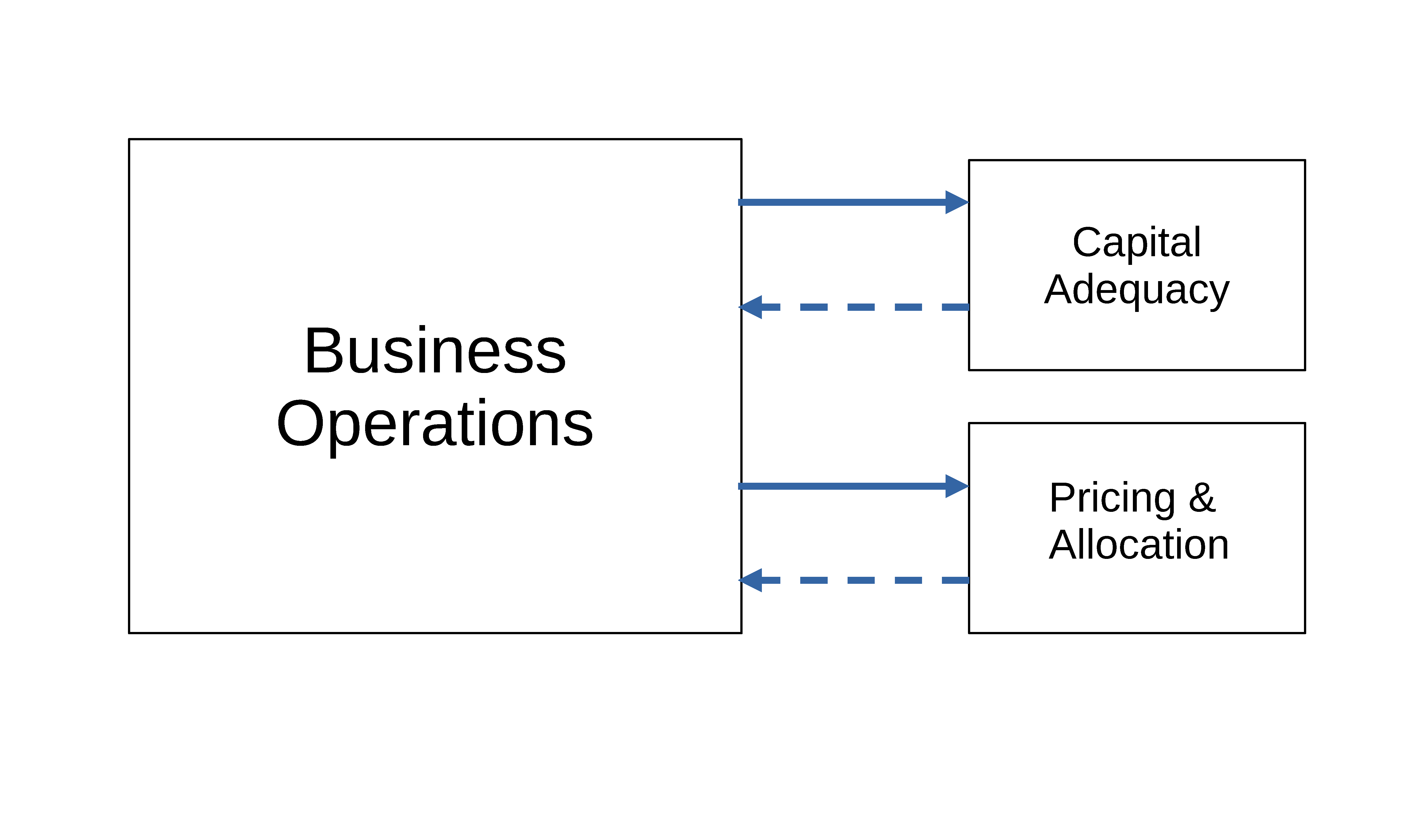
We can mentally decompose a capital modeling system into three components shown in Figure 1.1. By far, the biggest and most complex module represents the stochastic business of an insurer. This is labeled Business Operations in the diagram. A capital modeling system must represent some or all of the firm’s portfolio of insurance liabilities.
There is a wide range of sophistication possible to this representation, depending on the particulars of the purpose for which the system is to serve. The core concept is the loss which the portfolio might incur. This loss, being a priori uncertain, is a random variable. It might be represented by a distribution of losses or by a set of loss scenarios, which we will call events. The output could include just the losses, or it could include a complete set of financial statements—balance sheet, income statement, and cash flows—all of which ultimately depend on the losses. If the latter, there are numerous accounting standards that could be followed. These possibilities are discussed in Chapter 2.
Output from the Business Operations module feeds into the much simpler Capital Adequacy and Pricing & Allocation modules. This is signified by the solid arrows. Dotted arrows signify that these two modules, in turn, affect business operations in the real world and hence, indirectly, the Business Operations module. Indeed, the real-world effect of these modules is the raison d’être of the entire capital modeling system.
Figure 1.2 expands the Business Operations module.
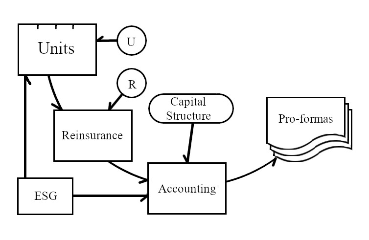
Starting at the left of the diagram is the Units module, with inputs labeled U. We use the term “unit” to refer to a component of the portfolio. A unit can be a single policy or a group of policies defined by line of business, geography, branch, business unit, or other characteristics. A unit can also represent the segmentation between ceded and assumed reinsurance.
The output of Units is a representation of experience, which means paid loss, at the very least, but could also include a time series of loss developments, reserves, etc. Input parameters are things like exposure and possibly shape parameters for loss distributions.
These loss outputs are likely to be correlated (not independent) across the units either by common economic or social factors or enforced correlation via copulas, Iman-Conover sampling (Section 8.2), etc.
If investment experience is included as one (or more than one) unit, then input from the Economic Scenario Generator (labeled ESG) will be important. This is an optional module which represents external economic factors such as interest rates, returns on various asset classes, rates of monetary inflation, unemployment, etc.
The Reinsurance module, with inputs labeled R, modifies the gross experience of the units. This includes all outward (ceded) reinsurance. Any inward (assumed) reinsurance would be represented among the units. The output, net experience, includes the effect of any retrocession.
Accounting translates experience realizations into pro formas, i.e., financial statements. This output from the Accounting module is a core element of the system. Multiple occurrences of pro formas, generated on the fly or possibly stored in a database, are used in stochastic simulation, whereas single occurrences are used for analyzing specific events. The level of detail here must match the specification of the units.
The system is likely to include the input labeled Capital Structure. This specifies, at the very least, the total amount of assets available to pay claims. It may also specify details of noninsurance liabilities, such as bonds, preferred stock, and equity issued by the firm. The Economic Scenario Generator may have some influence on the outward cash flows—which reduce assets—from preferred and common stock dividends. The Accounting module would take into account the fact that losses in excess of total assets lead to insolvency and haircuts in claim payments. If there is no capital structure information at all, asset limitations are ignored and assets are in effect assumed to be infinite.
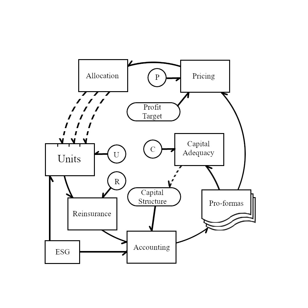
Figure 1.3 expands the picture by bringing in the remaining modules.
The Capital Adequacy module, with inputs labeled C, operates on the pro formas and determines the minimal amount of assets to satisfy requirements from regulators, rating agencies, and the risk committee of the firm’s board of directors. Such determinations could include a simple Value at Risk (VaR) calculation or more complex Best’s Capital Adequacy Ratio (BCAR) calculation. The module also includes risk reports—analysis of what is driving the need for assets. The input parameters can be regarded as the firm’s risk tolerance, specifying what level of risk is acceptable for a given amount of capital or vice versa. Outputs feed back into the real world and implicitly affect the capital structure, hence the dotted line. This is discussed in more detail in Chapter 3.
The Pricing module has two separately identified inputs. First, the Profit Target specifies the desired overall profitability of the portfolio as a whole. This could be posed as an aggregate premium, margin, loss ratio, or return on capital; these are equivalent specifications discussed in Chapter 4. The second input, labeled P, specifies more esoteric properties such as the shape of the distortion function underlying an SRM—also discussed in Chapter 4. The two inputs can be interpreted as specifying the firm’s risk appetite.
Allocation takes the required portfolio premium as given and allocates the premium (equivalently margin, loss ratio) to the individual units. This information, presumably, has real-world impacts on the units via performance management, risk management, underwriting actions, etc. Impact is represented by the dotted arrows to Units.
1.6 Introduction to InsCo
InsCo is our one-period simplified model of insurance company operations.
We will use an extremely simple toy example to illustrate the operation of the system presented in Section 1.5. It deliberately abstracts away from much of the complexity, detail, and nuance of the real world. Readers should be able to reproduce the example easily in a spreadsheet.
A more complex and realistic example can be found in Section 9.5, and more in Mildenhall and Major (2022). Those, as well as this simple example and even more complex portfolios, can all be analyzed with aggregate, an open-source Python library Mildenhall (2024) that “builds approximations to compound (aggregate) probability distributions quickly and accurately.” Because aggregate uses Fast Fourier Transforms, it “delivers the speed and accuracy of parametric distributions to situations that usually require simulation” and is therefore much faster than simulation. All the analytical techniques discussed in this monograph can be implemented in aggregate.
InsCo is a limited liability company that intermediates between insureds and investors. InsCo’s customers are insureds (policyholders) who are subject to risks they wish to insure. Insureds who use insurance for risk transfer or financing are sensitive to insurer quality and possible default because it correlates with their own misfortune.
Insurance legal entities serve two principal purposes. First, they provide statutory insurance such as mandatory automobile liability. Second, they allow insureds to pool together and benefit from diversification without requiring onerous bilateral contracts. They do this through insolvency rules, which provide the framework under which unrelated insureds interact in the unlikely event of an insolvency.
InsCo comes into existence at time \(t=0\) and lasts for one period. InsCo has no initial liabilities. At \(t=0\), it writes one or more single-period insurance contracts and collects premiums from its insureds.
When InsCo writes a policy, it collects premium at \(t=0\) and earns it over the period. We assume all other transactions occur at the end of the period. Therefore all the premium is earned and available to pay claims at \(t=1\). If InsCo’s ending assets \(a\) are insufficient to pay the claims, then it defaults.
InsCo has promised to pay policyholders claims under various contingencies, with the aggregate promise represented by the random variable \(X\ge 0\). If \(X>a\), then only \(a\) gets paid out, i.e., the actual payments are the minimum of \(X\) and \(a\), which we write as \(X\wedge a\). We assume the probability distribution of \(X\) is known.
InsCo is owned by investors who provide risk-bearing capital. Investors are also risk averse. The market structure is displayed in Figure 1.4.

At time \(t=0\), while collecting premiums, InsCo also raises capital from investors by selling them its uncertain \(t=1\) residual value. That is, at time \(t=1\), InsCo pays any claims due in the amount of \(X \wedge a\) and pays any residual value \((X-a)^+\), if it exists, to its investors as return of capital plus a dividend or investment return. If InsCo’s ending assets are insufficient to pay the claims, \(X>a\), then it defaults. Investors have limited liability: they may lose their original investment but owe nothing more.
Premiums cover expected losses and loss adjustment expenses, as well as the cost of capital including frictional capital costs. All other expenses are outside our model.
Symbolically, at time \(t=0\), InsCo collects premiums \(P\) from policyholders and capital \(Q\) from investors. These are the only sources of funds and comprise the total assets via the funding equation: \[ a = P+Q. \tag{1.1}\] Two important questions arise from InsCo’s promises to pay.
- Are there sufficient assets to honor those promises?
- Are investors being adequately compensated for taking on those risks?
Crucially, we need to talk about not one but two different risk measures to answer these questions.
Question 1 concerns risk tolerance and is answered by the Capital Adequacy module. It determines the assets necessary to back an existing or hypothetical portfolio at a given level of risk. This exercise can also be reverse engineered: given existing or hypothetical assets, what constraints on business does the risk tolerance entail? Alternatively, given business and capital, what is the implied risk tolerance?
Assets \(a\) and liabilities \(X\) are related by some rule driven by a combination of regulatory authorities, rating agencies, and InsCo’s own internal risk management policies, representing a risk tolerance. Such a rule we call a capital risk measure, and we may write \(a\) as a functional \(a(X)\). Value at Risk (VaR) or Tail Value at Risk (TVaR) at some high confidence level, such as 99.5% or 1 in 200 years, are both popular, but other possible measures exist, see Chapter 3. As a first approximation, we may take it that \(a\) is sufficient to avoid insolvency altogether, i.e., in all events, all claims are paid.
Question 2, answered by the Pricing module, concerns how that asset amount \(a\) is to be split between premium \(P\) and capital \(Q\) (Equation 1.1); this is quite different from determining \(a\). It is about risk pricing or risk appetite. We must determine the expected margin insureds need to pay in total to make it worthwhile for investors to bear the portfolio’s risk. Such a rule we call a pricing risk measure, and we may write premium as a functional \(P = \rho(X)\).