5 Applications of pricing and allocation
Performance assessment, new business pricing, and reinsurance decision-making are all essentially the same exercise as price allocation. Mergers and acquisitions, and portfolio optimization, must be approached differently.
Table 5.1 summarizes the events affecting InsCo’s three units of business as well as an available 35 excess of 65 stop loss reinsurance cover. This has ceded losses of zero in events 0 through 6 and 35 in event 7. It has an expected payout of 3.5 (loss on line 10%) and ceded premium of 6.5 (rate on line 18.6%). The expected net profit to the reinsurer is 3.0.
In the last three rows of the table we see the expected loss, the plan premium, and the required premium as calculated by a Wang transform calibrated to achieve a 15% return on capital for the (gross) portfolio.
| \(k\) | \(p\) | Unit A | Unit B | Unit C | Gross | 35 xs 65 | Net |
|---|---|---|---|---|---|---|---|
| 0 | 0.0 | 0 | 0 | 0 | 0 | 0 | 0 |
| 1 | 0.1 | 15 | 7 | 0 | 22 | 0 | 22 |
| 2 | 0.1 | 15 | 13 | 0 | 28 | 0 | 28 |
| 3 | 0.1 | 5 | 20 | 11 | 36 | 0 | 36 |
| 4 | 0.4 | 10 | 24 | 6 | 40 | 0 | 40 |
| 5 | 0.1 | 26 | 19 | 10 | 55 | 0 | 55 |
| 6 | 0.1 | 17 | 8 | 40 | 65 | 0 | 65 |
| 7 | 0.1 | 16 | 20 | 64 | 100 | 35 | 65 |
| \(\mathsf E[X]\) | 13.400 | 18.300 | 14.900 | 46.600 | 3.500 | 43.100 | |
| Plan | 13.900 | 18.700 | 19.600 | 52.200 | 6.500 | 45.700 | |
| \(\rho_{Wang}\) | 14.109 | 18.637 | 20.819 | 53.565 | 6.087 | 47.478 |
5.1 Performance assessment
Which units are performing at a satisfactory level?
Performance assessment is a multiattribute question, involving:
- recent and prospective growth
- expense control
- employee turnover
- customer retention
- competitive standing
- product and operational innovation
and other qualities. However, a key factor is profitability. The first question is always: Is this unit meeting a profit benchmark?
Recall we have a 15% return benchmark for the (gross) portfolio as a whole. Table 5.1 shows that additional premium of \(53.565-52.2=1.365\) is required to meet this threshold. This is true independent of the choice of distortion function—it is a direct consequence of the 15% return on capital requirement. Here we assume a calibrated Wang transform is used to allocate the portfolio requirement down to the units.
Table 5.2 shows that of the three units, only Unit B has a plan premium that exceeds the allocated target premium, and there, only by 0.063. Unit A has a deficit of 0.209, and Unit C has most of the portfolio deficit at 1.219. Putting these shortfalls in perspective, Unit C still has the highest gap measured in loss ratio (4.45%), but Unit A needs to increase its plan margin by the greatest factor (41.8%)
| Metric | Unit A | Unit B | Unit C | Gross |
|---|---|---|---|---|
| Plan Premium | 13.900 | 18.700 | 19.600 | 52.200 |
| \(\rho_{Wang}\) | 14.109 | 18.637 | 20.819 | 53.565 |
| \(\mathsf E[X]\) | 13.400 | 18.300 | 14.900 | 46.600 |
| Plan margin | 0.500 | 0.400 | 4.700 | 5.600 |
| Excess margin | -0.209 | 0.063 | -1.219 | -1.365 |
| % of plan | -41.8% | 15.6% | -25.9% | -24.4% |
| Excess LR | -1.43% | 0.33% | -4.45% | -2.28% |
Note this analysis depends heavily on the fact that we have chosen the Wang transform to drive our SRM allocation. What if a different distortion function were used? And how do we decide which one to use? These questions are addressed in Chapter 8.
5.2 Reinsurance decision-making
Reinsurance serves as loss protection and a source of loss-bearing capital. Table 5.1 shows a 35 excess of 65 portfolio stop loss contract. We assume this is aggregate cover, so questions of reinstatement do not apply. Per-occurrence cover would need to be analyzed to see its impact on aggregate results.
Should this cover be purchased?
Reinsurance decisions must weigh several factors, including impact on capital requirements and underwriting constraints, counterparty credit risk, and price. First let us consider capital requirements.
Previously, we assumed a \(\mathsf{TVaR}_{0.99}\) standard for required assets. For the gross portfolio, this led to \(a=100\), full collateral in this example. For the net portfolio, it would lead to \(a=65\) if full credit were to be allowed or if the same standard were applied to net losses.
Exercise. Apply the rate of return-driven pricing formula (Equation 4.2) to derive the required premium for the net portfolio based on a 15% required return. What might you conclude about the price of the reinsurance cover?
Solution. \[ P = \nu L + \delta a = (0.86956)(43.1) + (0.13043)(65) = 45.956 \] where \(L=43.1\) is the net expected loss per Table 5.1, and \(a=65\) is the required asset conditional on having stop loss reinsurance. For comparison, recall from the end of Section 4.1 that \(P(gross) = 0.86956\cdot46.6+0.13043\cdot100=53.565\) (consistent with plugging in values from the Gross column of Table 5.1). This represents savings of 7.609, which is the maximum that InsCo should be willing to cede for the cover. Since the cover costs 6.5 (Table 5.1), we might conclude that the price of the cover is advantageously low and it should be purchased (unless a better deal were available).
Unfortunately, this line of thinking relies on the familiar CCoC assumption. The risk profile has changed between the gross and net portfolio, so there is no basis for assuming that the same rate of return is required. An alternative approach is to use the loss protection interpretation and view reinsurance as a source of capital. This is elaborated upon in Mildenhall and Major (2022).
Applying the same Wang transformation allocation to the reinsurance cash flows, Table 5.1 shows a target required premium of 6.087, which is 0.413 lower than the actual 6.5 ceded premium. We conclude the cover should not be purchased.
Exercise. Using the Wang allocation and assuming \(a=65\), compute the return on capital for the net portfolio. Explain why the result is in this direction.
Solution. \[ \iota = \frac{M}{Q} = \frac{P-L}{a-P} = \frac{47.478-43.1}{65-47.478} = \frac{4.378}{17.522} = 25\%. \] All investment tranches \((Q_j^{Net},M_j^{Net})=(Q_j^{Gross},M_j^{Gross})\), \(j=1,\dots,5\) are identical, but the last tranche \(j=6\) has \(\Delta X_j^{Net}=0 < \Delta X_j^{Gross}\). Relative to gross, the net WACC is therefore skewed to the lower tranches, which have higher exceedance probabilities and therefore higher required returns.
5.3 New business pricing
While underwriting involves many factors other than pricing, such as exposure guidelines and physical and financial standards reflecting moral hazard, etc., pricing is a key task in the onboarding of new business.
At first glance, this seems equivalent to the performance assessment task: calculating a required premium as a distorted loss expectation. It would seem there is not much to add to this discussion. Typically, however, proposed new business is not run through the full capital model directly because that would be inefficient in terms of computing resources and timeliness. Rather, a simplified or surrogate version of the capital model is used to extract key loss statistics.
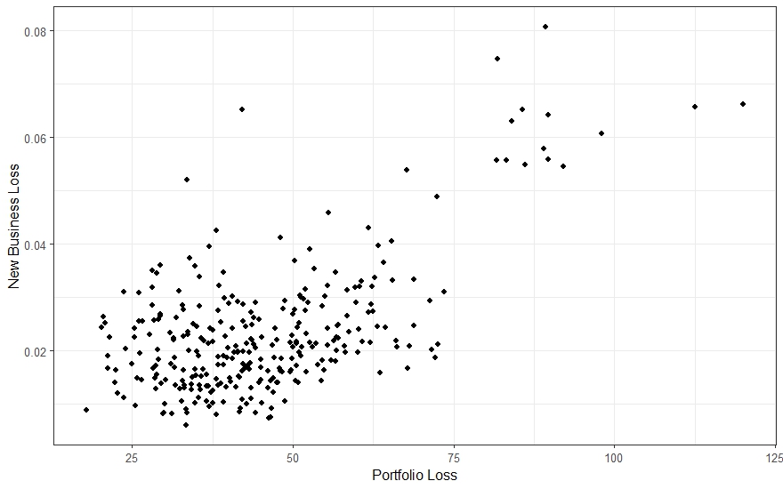
Let’s say for example we have a (relatively) simple cat model through which the portfolio has been run—once, and the results stored—and through which a new business prospect has just been run. Non-cat losses are represented by an independent lognormal variable calibrated on exposure characteristics. The resulting scatter plot is shown in Figure 5.1.
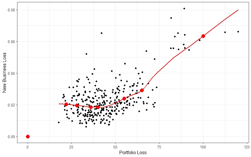
The problem is to translate these results into a form suitable for SRM allocation pricing. One could use the calibrated Wang transform to sort these results by the portfolio loss and calculate distorted probabilities, but we have no guarantee that the surrogate model accurately reproduces the distribution of portfolio losses that the capital model uses. The solution is to extract the conditional expected new business losses for each portfolio loss in Table 5.1. (See the discussion of \(\kappa^i(X_k)\) in Section 4.3).
This extraction can be done via local regression (LOWESS, LOESS, kernel smoothing; Friedman et al. (2008)). Figure 5.2 shows the scatter plot of Figure 5.1 with an estimate of the conditional mean loss curve and the specific event points. This leads to the augmented loss (Table 5.3).
| \(k\) | \(p\) | \(q\) | Gross | New Business |
|---|---|---|---|---|
| 0 | 0.0 | 0.0000 | 0 | 0.00000 |
| 1 | 0.1 | 0.0522 | 22 | 0.02028 |
| 2 | 0.1 | 0.0660 | 28 | 0.01965 |
| 3 | 0.1 | 0.0748 | 36 | 0.01849 |
| 4 | 0.4 | 0.3791 | 40 | 0.01855 |
| 5 | 0.1 | 0.1190 | 55 | 0.02402 |
| 6 | 0.1 | 0.1350 | 65 | 0.02910 |
| 7 | 0.1 | 0.1739 | 100 | 0.06339 |
| \(L=\mathsf E[X]\) | 46.600 | 0.02491 | ||
| \(P=\rho_{\mathsf{Wang}}(X)\) | 53.565 | 0.02858 | ||
| \(M=P-L\) | 6.965 | 0.00367 |
Exercise. Why is it reasonable to treat a small new business addition as if it were a unit within the portfolio, using the SRM allocation to calculate a reservation price?
Solution. Because it would have little or no impact on the sort order of portfolio losses. The distorted event probabilities \(q\) are functions of the distorted exceedance probabilities \(g(S)\), which are in turn functions of exceedance \(S\), which in turn is crucially dependent on the sort order of portfolio event losses. In the simple example, adding the new business losses \(X^{n}\) to portfolio losses \(X\) did not change the sort order of \(X+X^{n}\) compared to \(X\). In general, with a realistically fine-grained simulation, there may indeed be changes in the sort order, but they will be small and not be material to the results.
5.4 Mergers and acquisitions
What do you need to consider in a merger or acquisition? In general, there are quite a few considerations, such as strategic fit, financial performance of the target company, cultural compatibility, synergies and cost savings, regulatory compliance, tax implications, valuation for the target company, and risk management.
While the finance department will no doubt have an opinion on valuation, the capital modeling team could also be tasked with an analysis of how the risk profile of the new portfolio fits with the existing portfolio. The same principles discussed previously still apply, but with a twist. Whereas it was reasonable to treat a new business policy as if it were already a (relatively small) unit within the portfolio, a sizeable acquisition requires a different approach.
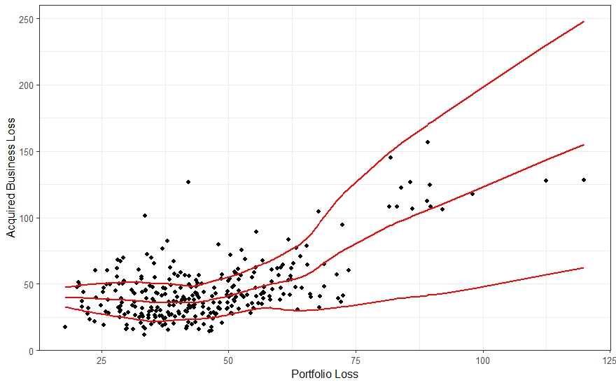
Say instead of the loss distribution portrayed in Figure 5.1, we had an acquisition opportunity with losses scaled up nearly 2,000 times larger on the \(y\)-axis at every point, having a mean loss of 48.35. We will focus on losses, with the acquired premiums to be compared to the required premium we will calculate.
Rather than the conditional mean loss of the acquired business (hereinafter \(X^a\)), we need the entire conditional distribution (or at least a representative sample). There are several technical approaches to this, such as quantile regression (Koenker and Hallock 2001) or kernel smoothing (Wand and Jones 1994). For our example, we will take what is possibly the simplest nontrivial approach.
- Calculate the conditional mean \(\bar{X^a} = \mathsf E[X^a|X]\) via LOWESS at every \(X\) point in the scaled-up equivalent to Figure 5.1, just as we did to obtain Figure 5.2.
- At each such \(X\) point, compute the squared difference between \(X^a\) and \(\bar{X^a}\).
- Use LOWESS again to compute the conditional mean square deviation, i.e. the variance, and its square root, the conditional standard deviation, \(\sigma_a\).
- Inspired by Gauss-Hermite quadrature (Kovvali 2022), we compute \(\bar{X^a}\) plus or minus one standard deviation. This is depicted in Figure 5.3.
- Duplicate each row in Table 5.1, inserting a new column for loss \(X^a\) consisting of those \(\bar X^a \pm \sigma_a\) points. Rescale each probability by half.
- Insert a new column for merger losses \(X^m=X+X^a\). Sort on \(X^m\).
- Compute \(S\), \(g(S)\), and \(q\) as before, based on the same Wang transform SRM. This is shown in Table 5.4.
| \(k\) | \(p\) | \(X\) | \(X^a\) | \(X^m\) | \(S\) | \(g(S)\) | \(q\) |
|---|---|---|---|---|---|---|---|
| 0 | 0 | 0 | 0 | 0 | 1 | 1 | 0 |
| 1 | 0.05 | 22 | 29.37 | 51.37 | 0.95 | 0.9766 | 0.0234 |
| 2 | 0.05 | 28 | 25.47 | 53.47 | 0.9 | 0.9478 | 0.0287 |
| 3 | 0.05 | 36 | 21.55 | 57.55 | 0.85 | 0.9161 | 0.0318 |
| 4 | 0.2 | 40 | 22.74 | 62.74 | 0.65 | 0.7667 | 0.1494 |
| 5 | 0.05 | 22 | 49.35 | 71.35 | 0.6 | 0.7244 | 0.0423 |
| 6 | 0.05 | 28 | 50.79 | 78.79 | 0.55 | 0.6802 | 0.0442 |
| 7 | 0.05 | 55 | 30.83 | 85.83 | 0.5 | 0.6341 | 0.0461 |
| 8 | 0.05 | 36 | 50.22 | 86.22 | 0.45 | 0.5859 | 0.0482 |
| 9 | 0.2 | 40 | 49.27 | 89.27 | 0.25 | 0.3700 | 0.2159 |
| 10 | 0.05 | 65 | 29.89 | 94.89 | 0.2 | 0.3089 | 0.0611 |
| 11 | 0.05 | 55 | 62.38 | 117.38 | 0.15 | 0.2439 | 0.0650 |
| 12 | 0.05 | 100 | 47.73 | 147.73 | 0.1 | 0.1739 | 0.0700 |
| 13 | 0.05 | 65 | 83.06 | 148.06 | 0.05 | 0.0964 | 0.0775 |
| 14 | 0.05 | 100 | 198.30 | 298.30 | 0 | 0 | 0.0964 |
| \(L=\mathsf E[X]\) | 46.60 | 48.35 | 94.95 | ||||
| \(P=\rho_{\mathsf{Wang}}(X)\) | 52.74 | 59.09 | 111.83 |
The required premium split between our original portfolio \(X\) (52.74) and the acquired \(X^a\) (59.09) is irrelevant to this analysis! Recall the original portfolio required premium was 53.57. What is important is the difference between the new merger portfolio premium 111.83 and the original premium of 53.57, i.e., 58.26. This is what InsCo would require for premium from the new business to secure enough margin to satisfy investors.
Exercise. Explain the capital situation. What increment of assets is needed with the newly acquired business? What capital? What is the total return on capital for the combined business? Return on incremental capital? Explain why this is not the 15% return originally specified.
Solution. Using a 95% TVaR criterion, total assets of 298.30 are needed for the combined portfolio, which is an increase of 198.30 over the original 100. With required premium of 111.83, this corresponds to capital of 186.46 for the combined portfolio, an increase of 140.03 over the original 46.43 (\(=100 - 53.57\)) capital. Margin on the combined portfolio is 16.88, for a return of 9.06%. The margin has gone up by 9.92, corresponding to a return of 7.08% on incremental capital. More capital is backing more remote probability losses, requiring less margin and therefore lower returns on capital.
5.5 Portfolio optimization
If this is the best of possible worlds,
what then are the others?
- Voltaire, “Candide”
5.5.1 Theory
Portfolio management is an inverse problem to pricing. Rather than taking the portfolio as given and determining appropriate pricing, the problem becomes to take the pricing as given and determine the best (or at least a better) composition of the portfolio. This task is typically complicated, however, by constraints such as volume or risk measures.
The textbook approach to optimization (e.g., Postek et al. (2024b), available online at Postek et al. (2024a)) starts with an objective function \(f(x)\) where \(x\) is typically a vector parameter. The problem is to find the value of \(x\) that maximizes (or minimizes) \(f(x)\). This is often complicated by the existence of multiple constraint functions \(h_j(x)\) requiring \(h_j(x) \le 0\) for \(j=1,\dots,n\) and \(h_j(x) = 0\) for \(j=n+1,\dots,m\).
What should be our objective function? It is tempting to think it should be margin, the difference between plan premium and expected loss. However, if our revelations in Chapter 4 taught us anything, it is that modifying the portfolio will modify the risk and that being properly rewarded for risk goes beyond expected loss. We need to compare the (rescaled) plan premium to the (rescaled) required premium from the pricing functional.
We found at the end of Section 4.1 that InsCo’s economic value added (EVA) is \(-1.6\). Our goal will be to make EVA as large (positive) as possible, or at the very least make it less negative.
For portfolio optimization, the particulars will likely look like:
- Objective function is economic value added.
- The parameters are scale factors, one for each unit.
- The primary constraint is to stay at the current capital.
- Secondary constraints are limits on growing or shrinking each unit.
Scale factors determine the volume of each unit. The current portfolio includes the random variable \(X^i\) representing the losses from unit \(i\). We now introduce the random variable \(X^i(\epsilon)\) to represent its losses if the unit volume has changed by the factor \(1+\epsilon\). The original portfolio loss variable is \(X=\sum_i X^i(0)\) in this notation. If unit \(i\) were to grow, say, 5%, its loss random variable would be represented as \(X^i(0.05)\).
Let the portfolio loss random variable be \(X(\epsilon^1,\dots)=\sum_i X^i(\epsilon^i)\) and denote the corresponding required assets by \(a(\epsilon^1,\dots)\). For any particular \(\epsilon\) values, the capital model can compute these.
For the InsCo example, we will assume the constraints are \(-0.5 \le \epsilon \le 0.5\).
If unit losses scaled linearly, as they do in stock portfolios, then we would have \(X^i(\epsilon)=(1+\epsilon) X^i(0)\). Unfortunately, this is usually not the case with insurance, although catastrophe cover in a limited geographic area comes close. However, a properly defined scale factor will give us scaling in planned premium.
There is a second source of nonlinearity here. As units grow or shrink, so do their losses in each event. Because the computation of the pricing SRM (and probably the capital measure as well) depends on the ordering of portfolio losses, that ordering may change, and so the measure will vary nonlinearly with the scale factors. For small changes in scale (i.e. \(\epsilon\) close to 0), this reordering may not happen or may not make a material difference. Our approach will take this into account.
The primary capital constraint listed above needs elaboration. As the portfolio composition shifts, the asset requirement (specified by the capital risk measure \(a(X)\)) will change. So will the total plan premium. We interpret the constraint to mean that the portion of assets not supplied by premium, \(Q=a-P\) (Equation 1.1), be maintained at the current level. The constraint might have been simply not to exceed the current level, but we don’t want to “leave money on the table” in the sense of holding more capital than we are currently using to support risk. So the constraint is an equality. In some other application, there could be a target capital different than the current level. Our approach is easily adaptable to that.
In a real application, there might be other constraints. For example, we might not want total portfolio margin to go down. We will keep the example here relatively simple.
If EVA and required assets scaled linearly, then the above would be a linear programming (LP) problem that could be solved with readily-available linear programming codes. Locally, that is to say with \(\epsilon\) close to zero, this should be a good approximation. However, we want to handle bigger steps correctly, so we need a nonlinear optimization strategy. The Nelder-Mead Simplex algorithm is generally applicable, but its performance may suffer in comparison to methods that use first derivatives such as the conjugate gradient algorithm by Polak and Ribiere and the quasi-Newton method of Broyden, Fletcher, Goldfarb, and Shanno. Other methods, such as the Newton conjugate gradient algorithm, use both first and second derivatives.
In Python, these and other methods are available in scipy.optimize. In R, the same holds for nloptr. Some of these implementations rely on FORTRAN codes written half a century ago!
If we treat losses as scaling linearly, then we can make use of first derivatives in our solution method. First derivatives are almost automatically provided when the objective—portfolio EVA—is evaluated. Second derivatives are impractical to compute here. If we do not wish to treat losses as scaling linearly, then we have a few options:
- Use a method like Nelder-Mead that does not require derivatives.
- Compute derivatives numerically by evaluating the objective at nearby points. This could be computationally inefficient.
- Use a proxy model—a simpler version of the complete model that approximates it—to provide derivatives. This is essentially what we are doing when we assume linear scaling, but a more accurate nonlinear proxy might be available.
The overall solution strategy here is stepwise hill climbing:
- Identify promising directions for scale changes.
- Select new scale parameters satisfying the capital and scale constraints.
- Rerun the model at the new scales.
- Repeat until EVA improvement seems impossible.
With linear scaling, the important thing to remember is that allocated quantities (premium, assets, capital) are the same as marginal quantities. If a unit is scaled up by 1% (\(\epsilon=0.01\)), say, then the allocated quantity will go up by 1%.
5.5.2 InsCo optimization
The input data for InsCo is provided in Table 5.5.
| Quantity | Unit A | Unit B | Unit C | Portfolio |
|---|---|---|---|---|
| Plan premium \(P_P\) | 13.9000 | 18.7000 | 19.6000 | 52.2000 |
| Required prem \(P_R\) | 14.1092 | 18.6375 | 20.8186 | 53.5652 |
| EVA \(V=P_P-P_R\) | -0.2092 | 0.0625 | -1.2186 | -1.3652 |
| Required assets \(a\) | 16.0000 | 20.0000 | 64.0000 | 100.0000 |
| Plan capital \(Q_P=a-P_P\) | 2.1000 | 1.3000 | 44.4000 | 47.8000 |
| EVA/capital ratio \(r=V/Q_P\) | -0.0996 | 0.0481 | -0.0274 | |
| Minimum scale \(\epsilon_-\) | -0.5 | -0.5 | -0.5 | |
| Maximum scale \(\epsilon_+\) | 0.5 | 0.5 | 0.5 |
Exercise. Assume that event 10 is always the one to produce the largest portfolio loss and therefore the capital measure. Compute an expression for \(\epsilon^3\) (Unit C) in terms of \(\epsilon^1\) (Unit A) and \(\epsilon^2\) (Unit B) so that the capital equality constraint is maintained.
Solution. Plan capital is the difference between assets and plan premium (Equation 1.1). Given the event 10 assumption, both scale linearly in \(\epsilon\), so \(Q\) does as well. The requirement is \[ 47.8 = \sum_{i} Q_P^i(1+\epsilon^i) = 2.1(1+\epsilon^1) + 1.3 (1+\epsilon^2) + 44.4(1+\epsilon^3) \] therefore \[ \epsilon^3 = -\frac{2.1}{44.4}\epsilon^1 - \frac{1.3}{44.4}\epsilon^2 = -0.047297\epsilon^1 - 0.029279\epsilon^2. \]
A naive approach to optimization might take the linear approximation at face value and take the biggest and most advantageous change in scale parameters possible. Let’s see how this plays out with InsCo.
- The most advantageous first move is to reduce Unit A by 50%. This increases EVA by \((-0.2092) \cdot (-0.5) = 0.1046\). It also changes capital by \((2.1) \cdot (-0.5) = -1.05\).
- Now we need to increase overall writings to use up all available capital and get it back to the target. Unit B has a positive EVA/capital ratio and Unit C a negative, so Unit B has the most advantage. We would have to increase Unit B’s scale by \(1.05/1.3 = 0.808\) to completely use the capital, but this is outside the constrained range. Scaling by the max allowed 50% adds \(1.3 \cdot 0.5 = 0.65\) to the capital, bringing the net position to \(-1.05 + 0.65 = -0.4\). It also brings the EVA up by \(0.0625 \cdot 0.5 = 0.0313\) to \(0.1358\).
- We need a further adjustment, and the only candidate left is Unit C. Here we need a scale change of \(0.4/44.4 = 0.0090\), which is well within the allowed range. (The formula from the previous exercise tells us the same thing.) That brings the change in capital back to zero but changes EVA by \((-1.2186) \cdot 0.0090 = -0.0110\) for a net EVA of \(-1.2403\) and an improvement of \(0.1249\). Adding these predicted changes to the original figures gives the results in Table 5.6.
| Quantity | Unit A | Unit B | Unit C | Portfolio |
|---|---|---|---|---|
| Scale change \(\epsilon^i\) | -0.5 | 0.5 | 0.009 | |
| Plan premium \(P_P\) | 6.9500 | 28.0500 | 19.7766 | 54.7766 |
| Required prem \(P_R\) | 7.0546 | 27.9562 | 21.0061 | 56.0169 |
| EVA \(V=P_P-P_R\) | -0.1046 | 0.0938 | -1.2295 | -1.2403 |
| Required assets \(a\) | 8.0000 | 30.0000 | 64.5766 | 102.5766 |
| Plan capital \(Q_P=a-P_P\) | 1.0500 | 1.9500 | 44.8000 | 47.8000 |
Now, had these moves been limited to, say 2%, we might be satisfied to stop here. In a real application, such a schedule of scale changes would be scrutinized for other business factors and questions of implementation feasibility. Some targets would probably be modified; for example, the Unit C scale change would no doubt be rounded to 1%.
However, with 50% scale changes, we need to be wary of nonlinear effects. Let us rerun the model at the new scales.
Our starting point is the original, 10-event loss distribution from Table 2.1. We multiply the losses in each column \(i\) by the scale factor \(1+\epsilon^i\), retabulate the portfolio total loss, and then sort on the portfolio loss. We apply the same asset metric—essentially the maximum loss—and the same Wang transform for pricing. We do not compute a new Wang parameter to obtain a 15% portfolio return. Rather, we use the same parameter because this represents the investors’ risk appetite. With a new loss distribution and new asset requirement, we do not expect the same required return. The new loss table is set out in Table 5.7. The first column shows the original sorted event number \(j\), highlighting the reordering that has occurred with the change in volume by unit, see Table 2.1. Events 3, 4, 5, 7, and 8 all move and are therefore given a different weight by the Wang distortion. This extensive reshuffling accounts for the large (relative to EVA) change in required premium shown in Table 5.8.
| \(j\) | \(p\) | Unit A | Unit B | Unit C | Portfolio | \(S\) | \(g(S)\) | \(q\) |
|---|---|---|---|---|---|---|---|---|
| 0 | 0 | 0 | 0 | 0 | 1.0 | 1.000 | 0.000 | |
| 1 | 0.1 | 7.5 | 10.5 | 0 | 18.0000 | 0.9 | 0.931 | 0.069 |
| 2 | 0.1 | 7.5 | 19.5 | 0 | 27.0000 | 0.8 | 0.851 | 0.080 |
| 7 | 0.1 | 7.5 | 24.0 | 9.0811 | 40.5811 | 0.7 | 0.766 | 0.086 |
| 5 | 0.1 | 6.5 | 30.0 | 7.0631 | 43.5631 | 0.6 | 0.675 | 0.091 |
| 3 | 0.1 | 2.5 | 30.0 | 11.0991 | 43.5991 | 0.5 | 0.579 | 0.096 |
| 6 | 0.1 | 2.5 | 40.5 | 8.0721 | 51.0721 | 0.4 | 0.479 | 0.101 |
| 8 | 0.1 | 13.0 | 28.5 | 10.0901 | 51.5901 | 0.3 | 0.373 | 0.106 |
| 4 | 0.1 | 3.5 | 49.5 | 0 | 53.0000 | 0.2 | 0.261 | 0.112 |
| 9 | 0.1 | 8.5 | 12.0 | 40.3604 | 60.8604 | 0.1 | 0.140 | 0.121 |
| 10 | 0.1 | 8.0 | 30.0 | 64.5766 | 102.5766 | 0 | 0.000 | 0.140 |
| Quantity | Unit A | Unit B | Unit C | Portfolio |
|---|---|---|---|---|
| Scale change \(\epsilon^i\) | -0.5000 | 0.5000 | 0.0090 | |
| Plan premium \(P_P\) | 6.9500 | 28.0500 | 19.7766 | 54.7766 |
| Required prem \(P_R\) | 6.8115 | 28.6040 | 20.8271 | 56.2426 |
| EVA \(V=P_P-P_R\) | 0.1385 | -0.5540 | -1.0505 | -1.4660 |
| Required assets \(a\) | 8.0000 | 30.0000 | 64.5766 | 102.5766 |
| Plan capital \(Q_P=a-P_P\) | 1.0500 | 1.9500 | 44.8000 | 47.8000 |
| EVA/capital ratio \(r=V/Q_P\) | 0.1319 | -0.2841 | -0.0234 |
The final EVA of \(-1.466\) is not only not as good as the predicted \(-1.240\); it is worse than the original \(-1.365\). Such is the curse of nonlinearity. Studying the derivatives here, it seems we need to go backwards, increasing the scale of Unit A and decreasing Unit B.
If we run the model with Unit B rescaled at many points throughout the \([-0.5, 0.5]\) range, we obtain the results shown in Figure 5.4. Nonlinearity is obvious. This is why most optimization algorithms take relatively small steps when updating parameters.

Applying the Nelder-Mead Simplex algorithm, we obtain the surprising result that the scale constraints are not binding at the optimal solution. Unit A is to be reduced by almost, but not quite, 50%. Unit B is to be reduced by almost 21%. Details are in Table 5.9.
| Quantity | Unit A | Unit B | Unit C | Portfolio |
|---|---|---|---|---|
| Scale \(\epsilon^i\) | -0.478165 | -0.209790 | 0.028758 | |
| Plan premium \(P_P\) | 7.253507 | 14.776927 | 20.163665 | 42.194098 |
| Required prem \(P_R\) | 7.269164 | 14.816395 | 21.453658 | 43.539217 |
| EVA \(V=P_P-P_R\) | -0.015658 | -0.039468 | -1.289993 | -1.345119 |
| Required assets \(a\) | 8.349360 | 15.804200 | 65.840538 | 89.994098 |
| Plan capital \(Q_P=a-P_P\) | 1.095854 | 1.027273 | 45.676874 | 47.800000 |
| EVA/capital ratio \(r=V/Q_P\) | -0.014288 | -0.038420 | -0.028242 | -0.080950 |
A grid search shows the situation in the neighborhood of the solution. See Figure 5.5. The optimal point has an EVA value of \(-1.345\). The innermost contour represents an EVA level set of \(-1.350\). Parameters inside this contour get at least 75% of the way from the original EVA to the optimal EVA.

The solution suggests that Unit A and Unit B both need further reduction because of negative EVA. However, there is more going on here. Not only is there nonlinearity, there is discontinuity in first derivatives as evidenced by Figure 5.4. If we were to change the Unit B scale ever so slightly, from \(-0.20979\) to \(-0.209795\), we obtain dramatically different EVA allocations, Table 5.10.
| Quantity | Unit A | Unit B | Unit C | Portfolio |
|---|---|---|---|---|
| Scale \(\epsilon^i\) | -0.478165 | -0.209795 | 0.028759 | -0.659201 |
| Plan premium \(P_P\) | 7.253507 | 14.776834 | 20.163668 | 42.194008 |
| Required prem \(P_R\) | 7.334042 | 14.607535 | 21.597550 | 43.539127 |
| EVA \(V=P_P-P_R\) | -0.080535 | 0.169298 | -1.433882 | -1.345119 |
| Required assets \(a\) | 8.349360 | 15.804100 | 65.840548 | 89.994008 |
| Plan capital \(Q_P=a-P_P\) | 1.095854 | 1.027267 | 45.676880 | 47.800000 |
| EVA/capital ratio \(r=V/Q_P\) | -0.073491 | 0.164805 | -0.031392 | 0.059922 |
5.5.3 Summary
The term “portfolio optimization” is quite ambitious. There are some questionable assumptions that have to be imposed on the problem to get to a solution. There are inherent nonlinearities and discontinuous derivatives. The uncertainties (see Section 8.1) in the inputs and the underlying model itself no doubt add breadth to the range of near-optimal solutions. One should approach the task with a healthy dose of humility.
Perhaps the best that can be hoped for is to provide directions for portfolio improvement that are probably, approximately, correct.