| Ref | Variable or relationship | Interpretation |
|---|---|---|
| Monetary amounts | ||
| 1 | \(L\) | Expected loss |
| 2 | \(P\) | Premium |
| 3 | \(M\) | Margin |
| 4 | \(a\) | Total assets |
| 5 | \(Q\) | Capital |
| Related amounts | ||
| \(a-L\) | The unfunded liability above expected loss, funded by margin and capital | |
| Monetary identities | ||
| Prem | \(P=L+M\) | Premium is expected loss plus margin |
| Fund | \(a = P + Q\) | Funding equation: premium and capital only source of \(t=0\) assets |
| Ratios | ||
| 6 | \(\lambda = L/P\) | Loss ratio |
| 7 | \(\gamma = P/a\) | Premium to asset leverage (gamma=g for leveraGe) |
| 8 | \(\iota = M/Q\) | Expected return on capital (investor) or cost of capital (insured) |
| Related ratios | ||
| \(\nu = 1/(1+\iota)\) | Risk discount factor, analog of \(v=1/(1+i)\) | |
| \(\delta = \iota /(1+\iota)\) | Risk discount rate, analog of paying interest at \(t=0\) | |
| 7a | \(P/Q= \gamma/(1-\gamma)\) | Premium to capital leverage ratio, divide top/btm by \(a\), used Fund |
| Ratio identities | ||
| \(\delta = \iota \nu\) | Analog of \(d=iv\) in theory of interest | |
| Disc | \(1 = \nu + \delta\) | Analog to \(1=v+d\) |
| Capital identities | ||
| Q | \(Q=\nu(a-L)\) | \(Q\) is \(t=0\) price paid for asset with expected \(t=1\) return \(a-L\) |
| 8a | \(\iota = (P-L) / (a-P)\) | Substitute Prem and Fund into (8) |
| \(\delta = (P-L) / (a-L)\) | Substitute Prem and Fund into (8) | |
| Premium identities | ||
| P1 | \(P=\nu L + \delta a\) | Premium \(=\) weighted average of expected loss and maximum loss, \(a\) |
| P2 | \(P=a - \nu(a-L)\) | Premium \(=\) assets not funded by investor capital |
| P3 | \(P=L + \delta (a-L)\) | Premium \(=\) expected loss plus share of unfunded liability |
| P3a | \(P=L + \iota Q\) | As P3 but expressed in terms of cost of capital |
4 Pricing and allocation
This chapter is about the basic theory of allocating premium and capital based on the Natural Allocation of Spectral Risk Measures (SRMs). Here, we present the logic in an informal fashion. Think of it as the CliffsNotes or Schaum’s Outlines version. Topics include:
- the one-year InsCo model
- the relationship between assets, capital, and premium
- capital risk measures versus pricing risk measures
- portfolio pricing
- layer pricing
- event pricing
- unit pricing
- the constant cost of capital assumption.
Allocating capital per se is addressed in Section 8.3.
The theory presented here revolves around a one-period model. In reality, insurance claims often evolve over time with multiple payments spanning more than one accounting period. The output of the Business Operations module will undoubtedly reflect this. In order to apply the theory, we must collapse the multiperiod view into a single-period equivalent. There are two ways to do this. One, we can represent paid claims in a unit and carry a one-year change in reserves as a separate but parallel unit. Two, we can operate entirely in ultimate claims, discounting them back to time zero. To do this, we lean on the principles espoused in Wüthrich et al. (2010):
- If interest rates are not being modeled (you do not have an Economic Scenario Generator), use the latest available risk-free zero-coupon bond yield curve to discount future simulated paid claims to the baseline time in question.
- If an Economic Scenario Generator is available to generate random interest rates, use the generated zero-coupon bond yield curve in each event to discount payments in the same event.
Using risk-free rates to discount losses is somewhat controversial. Fairley (1979) argued for a risk-free rate because “policyholders do not share in [the insurer’s] investment risks…” Cummins (1990) argued for using the market return on the company’s actual portfolio because adding investment risk increases the probability of default for policyholders and therefore changes their expected loss recoveries, i.e., they do share in the investment risk. However, note that the insolvency priority order of payments puts policyholders first in line to be paid and shareholders last (i.e., first in line for losing money). Investment risk is not shared equally—if we want to follow Cummins’s line of reasoning, the correct discount rate for losses is nearer risk-free than it is the full investment yield. The risk-free rate is probably not a bad approximation.
An alternative theory is embedded in IFRS17 rules (Caramagno et al. 2021). There, a discount rate for future liability cash flows is the sum of a risk-free rate and a liquidity premium. Since insurance contracts cannot be traded continuously in a liquid market, investors must therefore demand a liquidity premium. Typically this is around 50 basis points. The IFRS17 rate proxies an entity independent market rate.
For more complex situations where cash flows depend more directly on financial outcomes (as is the case in much of life insurance), refer to Wüthrich et al. (2010)—but not the parts about risk loads; their approach is not the same as the SRM approach presented here!
4.1 Pricing the whole
Pricing applications of capital models typically proceed from the top down (Bühlmann 1985) and start by determining the premium needed for the whole portfolio to meet corporate return objectives. Total needed return depends on the amount of capital and the required return on that capital. Following the market structure laid out for InsCo (Figure 1.4), the amount is determined by regulators or rating agencies using a capital risk measure. The return is estimated using a separate analysis which will be used to calibrate the pricing risk measure.
A stock insurer uses a peer analysis of valuation against relevant financial metrics to estimate what it believes its investors require as a return on equity to support the current or desired share price. This return is combined with the capital structure (known debt costs) to determine a weighted average cost of capital across debt and equity, producing an implied needed total income. Income is then adjusted for non-underwriting income and taxes to determine needed income from insurance operations. It is this amount that is handed to the capital modelers to be allocated to individual units (Section 4.2). The analysis below ignores non-underwriting income and taxes and proceeds directly from the implied weighted average cost of capital. Mutual companies substitute their own analysis, reflecting their founding charter and mission, and their lack of access to equity financing, to determine an analogous cost of capital.
Say the analysis determines that investors require a 15% return on capital for their investment in InsCo. The portfolio’s premium, margin, capital, assets, and expected losses have a simple relationship with rate of return. The time value of money is ignored, i.e., the risk-free rate is zero. Here we analyze only the gross losses, leaving the analysis of reinsurance for later.
Define the expected loss \(L=\mathsf E[X\wedge a]\). \(L\) is slightly less than the promised loss \(\mathsf E[X]\) because of the possibility of default; in practice the adjustment is so small you can often ignore it. Premium can be decomposed into expected loss plus margin: \[ P=L+M. \tag{4.1}\] Equation 1.1, the funding equation, says \(a=P+Q\) giving the split of assets between policyholder premium and investor capital. Policyholders in aggregate have been promised \(X\) and investors the balance of funds \((a-X)^+\). If \(X>a\) policyholders are paid \(a\) and investors nothing. No matter the loss outcome, all ending assets are paid in losses or returned to investors: \[ a \equiv X\wedge a + (a-X)^+. \] Investors expect to receive \[ \mathsf E[(a - X)^+] = a - L = (P + Q) - L = (L+M) + Q - L = M + Q \] and therefore their expected return on investment is \(\iota=M/Q\).
In Chapter 10.5 of Mildenhall and Major (2022), we introduce the insurance pentagon, Figure 4.1, which displays key insurance pricing variables and the relationships between them. There are five monetary variables: premium, loss, margin, assets, and capital, and three ratios describing leverage, loss ratio, and return.

Table 4.1 displays a number of relationships between the eight key insurance variables which we use repeatedly: you should become familiar with them. The table uses Greek letters for the ratios and Roman for monetary amounts.
Premium (like discount) is received at \(t=0\), hence the relevance of \(\delta\). Income (like interest) is earned and paid at \(t=1\) and measured with \(\iota\). Discount is easier to work with as a measure of return because it is always between \(0\) and \(1\): \(\delta=1\) corresponds to an infinite return.
Pricing is the process of splitting the unfunded liability \(a-L\) into premium margin and capital parts funded by the policyholder and investor. The risk discount factors tell you how to accomplish this.
The relationship between premium and loss can be expressed using the loss ratio or its reciprocal, the premium multiplier. The latter is sometimes used in catastrophe pricing, when loss ratios seem embarrassingly low. Likewise, leverage could be expressed as premium to capital rather than as premium to assets. The point is there is a measure of leverage, a measure of margin to volume, and a measure of return-cost to capital.
Given required expected return from a top-down approach analysis, the standard pentagon equations in Table 4.1 show that knowing \(\iota\), \(L\), and \(a\) determines total premium. It can be expressed in multiple ways, the most helpful of which are \[ P = L + \delta (a-L) = L + \iota Q = \nu L +\delta a. \tag{4.2}\] The first two expressions make it clear that premium equals expected loss plus cost of capital. The third will reappear again and again in this monograph.
Example: TVaR Capital Risk Measure. Before considering allocation, let’s look at total pricing with a TVaR capital measure, \(a=\mathsf{TVaR}_p(X)\). The quantity \(a-L=\mathsf{TVaR}_p(X)-\mathsf E[X]\) is usually referred to as \(\mathsf{XTVaR}_p(X)\), for excess TVaR above the mean. Total premium, from Equation 4.2 becomes \[ \begin{aligned} P &= L + \delta (a-L) \\ %&= L + \delta (\mathsf{TVaR}_p(X) -L) \\ &= L + \delta \mathsf{XTVaR}_p(X) \\ &= L + \iota Q. \end{aligned} \]
Example: InsCo. Recall from Table 3.2 that the portfolio plan premium is 52.2. When \(\iota=0.15\), we have \(\nu=0.86956\) and \(\delta=0.13043\), resulting in a required portfolio premium of \(46.6+0.13043\cdot(100-46.6)=53.565\). The premium required to achieve a 15% return is 53.6, or 1.4 higher than plan. The required margin is 7.0, also 1.4 higher than the plan margin. This difference between plan and required profitability (negative here) is sometimes called Economic Value Added or EVA. It represents the amount of profit over and above what is required to satisfy investors. In Section 5.5 we see if we can improve the situation. In the rest of this chapter, we address how to allocate the required portfolio premium and margin to the units.
The pentagon contains eight variables and five relationships (funding, premium, loss ratio, leverage, and return) leaving three free variables, i.e., most of the time knowing three of the eight variables is enough to determine the rest. This sometimes fails, e.g., knowing the three ratios does not determine volume.
You should become familiar with the underlying algebra of Table 4.1, not memorize it, but be able to figure it out quickly. Here are some examples.
- Using \(\nu+\delta=1\) and starting from \(P=\nu L +\delta a\) gives \(P=(1-\delta)L + \delta a = L + \delta (a-L)\). Since we know \(P=L+M\), this implies \(M=\delta (a-L)\).
- Alternatively, \(P=\nu L + (1-\nu) a = a - \nu(a-L)\). Now, since we know \(a=P+Q\) so \(P = a-Q\), this implies \(Q=\nu (a-L)\).
- Hence return \(\iota = M / Q = \delta / \nu\).
Make sure you are happy with P3 and P3a. These are used repeatedly below.
4.2 Allocation to units: Overview
Introducing the Natural Allocation. The Natural Allocation (NA) is a way to allocate total premium or margin down to individual units. The method is natural because it relies on so few assumptions, is easy to compute, and gives a reasonable range of interpretable answers. It also agrees with the marginal and risk-adjusted probability methods when they are well defined—a huge conceptual advantage. The NA works by taking the problem of pricing the whole risk and dividing it into a series of simpler problems involving pricing individual layers of assets and then solving those simpler problems. Layers are easier to price because they are binary, involving no loss or a full loss, and are completely characterized by their probability of a loss. The NA is described in the next six sections.
- Section 4.3 describes four adjustments that must be made to raw simulated output before starting. These are technical, computational adjustments.
- Section 4.4 describes how the method works in total. It concludes by showing that the NA depends on the selection of a distortion function to determine the return to each layer of assets.
- Section 4.5 explains how to move from a total price for each layer to a price by layer by unit. Summing these allocations up across layers gives the unit NA.
- To this point, we have not introduced any distortion functions, so Section 4.6 introduces five families. These essentially span the full range of risk appetites. We compute the NA for the Wang distortion, which corresponds to a middle-of-the-road risk appetite.
- Section 4.7 describes how the NA works for the constant cost of capital distortion (CCoC) , which assigns the same return to each layer. The CCoC corresponds to a very extreme tail-risk averse risk appetite. Unfortunately, while the CCoC is an unrealistic assumption, it is the basis for what we call the industry standard approach. It is the root cause of many problems encountered in practical allocation work. We explain why and how it came to be accepted.
- Finally, Section 4.8 tries to head off objections to the NA caused by interpreting scenarios defined by outcome loss amount as events. If this idea has not occurred to you before already, we recommend skipping it! However, someone invariably brings it up, and you need to be able to explain why it is not a problem, so you do need to read it eventually.
4.3 Four technical adjustments
In order to make the algebra work out in subsequent sections, we need to adjust our events so that four simplifying conditions hold. These alter the form of the simulation data, but not the underlying meaning. We adjust our simulated loss outcomes so that
- Loss outcomes are sorted by total loss, from lowest to highest.
- The first loss is zero.
- Losses are capped at the available assets.
- Portfolio losses are unique by event.
Zero Loss. If, in our table of loss probabilities, the first, lowest, portfolio loss \(X_1\) is greater than zero (and this is true in Table 2.1), then it is computationally simpler to introduce another row with \(X_0=0\) and \(p_0=0\). This does not change the results because \(p_0=0\). If \(X_1=0\) already, then no such adjustment is necessary. However, in that case, we do renumber so that the first event is called \(k=0\). The reason for this will become apparent in the next section; layer size and exceedance probability must be properly accounted for.
Capped Losses. When there is zero probability of insolvency, allocating the portfolio’s expected loss \(\mathsf E[X]\) to unit \(i\) is easy—it’s just the unit’s expected loss \(\mathsf E[X^i]\). When assets are lower and there is a nonzero probability of default \(X>a\), we need to consider what actually happens to claim payouts. The most common rule, and the one we assume, is equal priority. Payments to unit \(i\) are given a common haircut: \[ \begin{aligned} X^i(a) :&= X^i \frac{X\wedge a}{X} \\ % &= \frac{X^i}{X} \, (X\wedge a)\\ &= \begin{cases} X^i & X \le a \\ X^i\dfrac{a}{X} & X > a. \end{cases} \end{aligned} \] This expresses payments to unit \(i\) as a constant pro rata (haircut) proportion \((X\wedge a)/X\) of the contractually promised payment \(X^i\). The factor is the same for all units, hence equal priority. We assume the appropriate substitutions have been made \[ \begin{aligned} X^i &\leftarrow X^i(a) \\ X &\leftarrow X \wedge a \end{aligned} \] in our loss table. It is important to realize that once this adjustment has been made we can ignore default. Default has not disappeared; by replacing promised loss payments \(X^i\) with actual \(X^i(a)\), we have “baked in” default. Going forward we can therefore ignore default as a separate phenomenon.
Unique Losses. Consider a particular outcome \(X=X_k\). If there is only one event with \(X=X_k\), then there is only one set of unit losses \(\{X_k^1,\dots,X_k^m\}\) whose sum is \(X_k\). If there are multiple events with \(X=X_k\) but the same set of \(\{X_k^i\}\) then we can, with no loss of information, collapse them all (summing the probabilities) and consider the result to be one event.
However, if there are two or more distinctly different events resulting in \(X=X_k\), then the above logic cannot be applied. This is true in Table 2.1. In this case marginal calculations do not make sense and, when, in Section 4.4, we go to distort probabilities, there will be an ambiguity in the ordering of the events which will be material to the calculations. We need to resolve that ambiguity, and we can do it by using the conditional expected loss of the units. Define \[ \kappa^i(x) := \mathsf E[X^i \mid X=x]. \] Then collapse the events sharing \(X=X_k\), replacing the particular \(X^i\) values with their conditional expectation \(\kappa^i(X_k)\) and summing the probabilities into the newly defined \(p_k\). We appeal to a symmetry argument: within the set of events resulting in \(X=X_k\), beyond their relative probabilities, there is no reason to prioritize one over another. Henceforth, we will assume the substitutions \[ X_k^i \leftarrow \kappa^i(X_k) \tag{4.3}\] have been made in our table of outcomes. Notice that Equation 4.3 always applies when losses exceed assets. The substitution Equation 4.3 relies on equal priority in the sense that the recovery to the collapsed event equals the conditional expectation of the recoveries to its components: \[ \begin{aligned} \mathsf E\left[X^i \frac{X\wedge a}{X} \mid X=x\right] &= \mathsf E\left[X^i \mid X=x\right]\frac{X\wedge a}{X} \\ &= \kappa^i(X) \frac{X\wedge a}{X}. \end{aligned} \] Thus, equal priority is essential to make the approach work. Luckily, equal priority is universal in insurance regulation, even though other approaches are possible in theory (Mildenhall and Major (2022), chapter 12.3).
In our example, notice in Table 2.1 that the events \(4\), \(5\), \(6\), and \(7\) all have \(X=40\). Taking the \(p\)-weighted averages of each unit’s losses across those events, collapsing the events down to one event, renumbering, and inserting the zero row, we get Table 4.2. The table has also added a row \(0\) with \(0\) loss and probability. There is no need for a default adjustment because \(a=100\), sufficient to pay the maximum loss.
| \(k\) | \(p\) | Unit A \(X^1_k\) | Unit B \(X^2_k\) | Unit C \(X^3_k\) | Portfolio \(X_k\) |
|---|---|---|---|---|---|
| 0 | 0 | 0 | 0 | 0 | 0 |
| 1 | 0.1 | 15 | 7 | 0 | 22 |
| 2 | 0.1 | 15 | 13 | 0 | 28 |
| 3 | 0.1 | 5 | 20 | 11 | 36 |
| 4 | 0.4 | 10 | 24 | 6 | 40 |
| 5 | 0.1 | 26 | 19 | 10 | 55 |
| 6 | 0.1 | 17 | 8 | 40 | 65 |
| 7 | 0.1 | 16 | 20 | 64 | 100 |
| \(\mathsf E[X]\) | 13.4 | 18.3 | 14.9 | 46.6 | |
| Plan Prem | 13.9 | 18.7 | 19.6 | 52.2 |
4.4 Pricing layers in total
Layer pricing assumes the required return associated with each individual dollar of assets is given by a function of its risk of being consumed for claim payments.
The NA is based on the principle of layer pricing, introduced formally by Wang (1996) and articulated by Venter (1991), Bodoff (2007), and others.
Suppose the total assets \(a\) are funded by premium and the sale of the residual value of separate layers or tranches. These layers are analogous to collateralized aggregate reinsurance, as we shall now explain. Reinsurance in our one-period model is a transaction where ceded premium is paid to the reinsurer at \(t=0\) and ceded losses are recovered from the reinsurer at \(t=1\). Let’s turn that around to make the role of reinsurance as capital more transparent. InsCo (or its regulator) demands collateralized reinsurance. Consider a layer of width \(\Delta X_k\). The layer has its own funding equation and needs to be supported by assets of \(\Delta X_k\) in total. At \(t=0\) the counterparty remits \(\nu (\Delta X_k-L_k)\) and the insurer \(L_k+\delta(\Delta X_k-L_k)\) into the collateral account, where \(L_k\) is expected loss in the layer. Since \(\nu+\delta=1\), the layer is fully collateralized. At \(t=1\) the layer loss becomes known and is paid in full from collateral. Any amounts remaining are remitted back to the counterparty. This is reinsurance, but with the transactions reversed to reveal the capital financing function.
To be concrete, say we understand the distribution of portfolio losses \(X\) through a simulation. Say the annual aggregate results \[ X \in \{X_0 < X_1 < \dots < X_n=a\} \] and each outcome has its probability \(\{p_0, p_1, \dots, p_n\}\).
We tranche total assets \(a\) into a stack of fully collateralized aggregate reinsurance layers. Each layer is a half-open interval, \(k=0,\dots,n-1\), covering losses \(X \in (X_k,X_{k+1}]\), i.e., for a loss of \(X\) it pays \[ \begin{cases} 0 & X \le X_k \\ X - X_k & X_k < X \le X_{k+1} \\ \Delta X_k & X_{k+1} < X \end{cases}. \] However, there are no partial payments because \(X_k\) are the only possible outcomes, so the cover reduces to one paying nothing when \(X \le X_k\) and \(\Delta X_k\) as soon as \(X > X_k\).
For our InsCo numerical example, \(X \in \{0, 22, 28, 36, 40, 55, 65, 100\}\) and \(n=7\). So, we have seven layers \((X_k, X_{k+1}]\) that we imagine are funded separately, each by a combination of investor capital (security market purchase price of the returned collateral) and insured’s premiums. The probability that losses exactly equal \(X_k\) is \(p_k\). The probability that layer \(k\) is used for loss payments (rather than handed back to investors) is the exceedance probability or survival function (hence notation \(S\)): \[ S_k = S(X_k) := \Pr\{X>X_k\} = \sum_{j=k+1}^n p_j. \] The numbers for our example are laid out in Table 4.3.
| \(k\) | \(p\) | Unit A \(X^1_k\) | Unit B \(X^2_k\) | Unit C \(X^3_k\) | Portfolio \(X_k\) | Layer size \(\Delta X_k\) | Exceedance Pr \(S_k\) |
|---|---|---|---|---|---|---|---|
| 0 | 0 | 0 | 0 | 0 | 0 | 22 | 1 |
| 1 | 0.1 | 15 | 7 | 0 | 22 | 6 | 0.9 |
| 2 | 0.1 | 15 | 13 | 0 | 28 | 8 | 0.8 |
| 3 | 0.1 | 5 | 20 | 11 | 36 | 4 | 0.7 |
| 4 | 0.4 | 10 | 24 | 6 | 40 | 15 | 0.3 |
| 5 | 0.1 | 26 | 19 | 10 | 55 | 10 | 0.2 |
| 6 | 0.1 | 17 | 8 | 40 | 65 | 35 | 0.1 |
| 7 | 0.1 | 16 | 20 | 64 | 100 | 0 | 0 |
How is layer \(k\) to be funded? Analogous to our portfolio funding Equation 1.1, we have the layer funding equation: \[ \Delta X_k = P_k+Q_k. \tag{4.4}\]
While the portfolio funding equation is self-evident, is it necessary to constrain a layer’s capital to \(Q_k=\Delta X_k-P_k\), or can it be something else? It is easy to see it cannot provided \(P = \sum_k P_k\). Let’s assume that (we’ll justify it later) and see why. First, note that \(Q_k\ge \Delta X_k - P_k\) for each \(k\), otherwise there could be a shortfall in loss payments on the layer. This is just the statement that each layer must be fully collateralized. Now, if the inequality is strict for any \(k\), we get \(Q=\sum_k Q_k > \sum_k \Delta X_k - P_k = a - P = Q\), which is a contradiction. Hence \(Q_k = \Delta X_k - P_k\).
We still need to justify \(P = \sum_k P_k\). You might think that the aggregate premium could be less than the sum of the premiums by layer because of potential diversification opportunities between the layers. However, in a sense there are no diversification opportunities between the layers because they are comonotonic: they are all increasing functions of the total loss \(X\). Some, but not all, pricing functionals are comonotonic additive, meaning that the price of the sum of comonotonic risks equals the sum of the prices. To proceed, we need to use a comonotonic additive pricing functional. This is not a problem, as the functionals we are proposing to use are comonotonic additive. Thus, we may assume the layer funding Equation 4.4 holds.
We have reduced the pricing problem to pricing a fully collateralized layer. Here again we can apply our general rules: if we know the expected loss and return by layer we know the premium. \(S_k\) is the probability that layer \(k\) is needed to pay claims and so \(L_k=S_k\Delta X_k\) is the expected value of layer \(k\)’s contribution to the total portfolio expected claim payments \(L\). For the return, we need to made one last assumption: \(S_k\) is the only thing that investors deem relevant to pricing layer \(k\). In layer \(k\), the investors get \(\Delta X_k\) back with probability \(1-S_k\) and nothing with probability \(S_k\). Layer \(k\)’s payoff as a fraction of its limit \(\Delta X_k\) is a Bernoulli random variable with one parameter: \(1-S_k\). We assume that its probability distribution, determined by \(S_k\), is all that matters. This restriction is known as law invariance.
A risk measure \(\rho(X)\) is law invariant if and only if it is a function of the distribution \(F\) of \(X\). That is, if \(X\) and \(Y\) have the same distribution function, then \(\rho(X)=\rho(Y)\). Law invariant risk measures do not depend on the cause of loss or the particulars of the event generating the loss. VaR, TVaR, and standard deviation are examples of law invariant risk measures. A measure like \(\rho(X)=\mathsf E[X] + \lambda \mathsf{cov}(X, Y)\), which depends on a state variable \(Y\), is not.
Law invariance may seem a strange assumption for a pricing risk measure, especially in the light of theories like the capital asset pricing model where systematic or nondiversifiable risk is considered (these are not law invariant). The rationale is that insurance risk is diversifiable and has no analog of market risk. The motivation for law invariance in the capital risk measure stems from a regulator’s desire for an objective default probability measure. An entity’s risk of insolvency depends only on the distribution of its future change in surplus—the cause of loss is irrelevant. Law invariance enables risk to be estimated statistically, from an empirical sample or a model fit to \(X\). Law invariance is sometimes called objectivity for these reasons. It allows regulators to calibrate their models using only losses. While the justification for law invariance in the pricing measure is admittedly weaker, we find it eminently useful.
Suppose we know (or, being actuaries, assume) a function \(g(s)\) that maps attachment probability \(S_k\) to rate on line (premium to limit ratio) allowing us to write \[ P_k = g(S_k)\Delta X_k. \] The function \(g(s)\) is known as a distortion function.
Before moving on, here is a summary of the key assumptions that we have made and how they are used:
- Equal priority in default – collapse equal outcomes to one.
- Comonotonic additive pricing risk measure – funding equation by layer.
- Law invariant pricing risk measure – price layer using a distortion function.
- Existence of a rate on line distortion function \(g\) for pricing Bernoulli layers.
Distortion functions must have certain properties if the layer prices are to be rational. In particular, \(g(0)=0\), \(g(1)=1\), and \(g\) must be increasing and concave (decreasing slope). Violations of these lead to irrational pricing behavior, as defined and explained in Mildenhall and Major (2022), chapter 10.
The logic for pricing layer \(k\) is exactly the same as what was used to derive Equation 4.2 and gives: \[ P_k = g(S)\Delta X_k = \nu_k S_k \Delta X_k +\delta_k \Delta X_k \tag{4.5}\] where the return \(\iota_k\) and risk discount factors \(\nu_k\) and \(\delta_k\), are functions of \(S\) (hence the subscripts). So, if we knew the required return \(\iota_k\) associated with layer \(k\), we could determine its premium and capital. Summing across all layers we would then know both total premium and total capital, and they would sum to total assets \(a\). Computing the total premium \[ P = \sum_j g(S_j)\Delta X_j \] in this way is known as a Spectral Risk Measure (SRM). SRMs are coherent risk measures in the sense of Artzner et al. (1999). They are also law invariant (of course) and comonotonic additive, and in fact are the only risk measures that have all these properties.
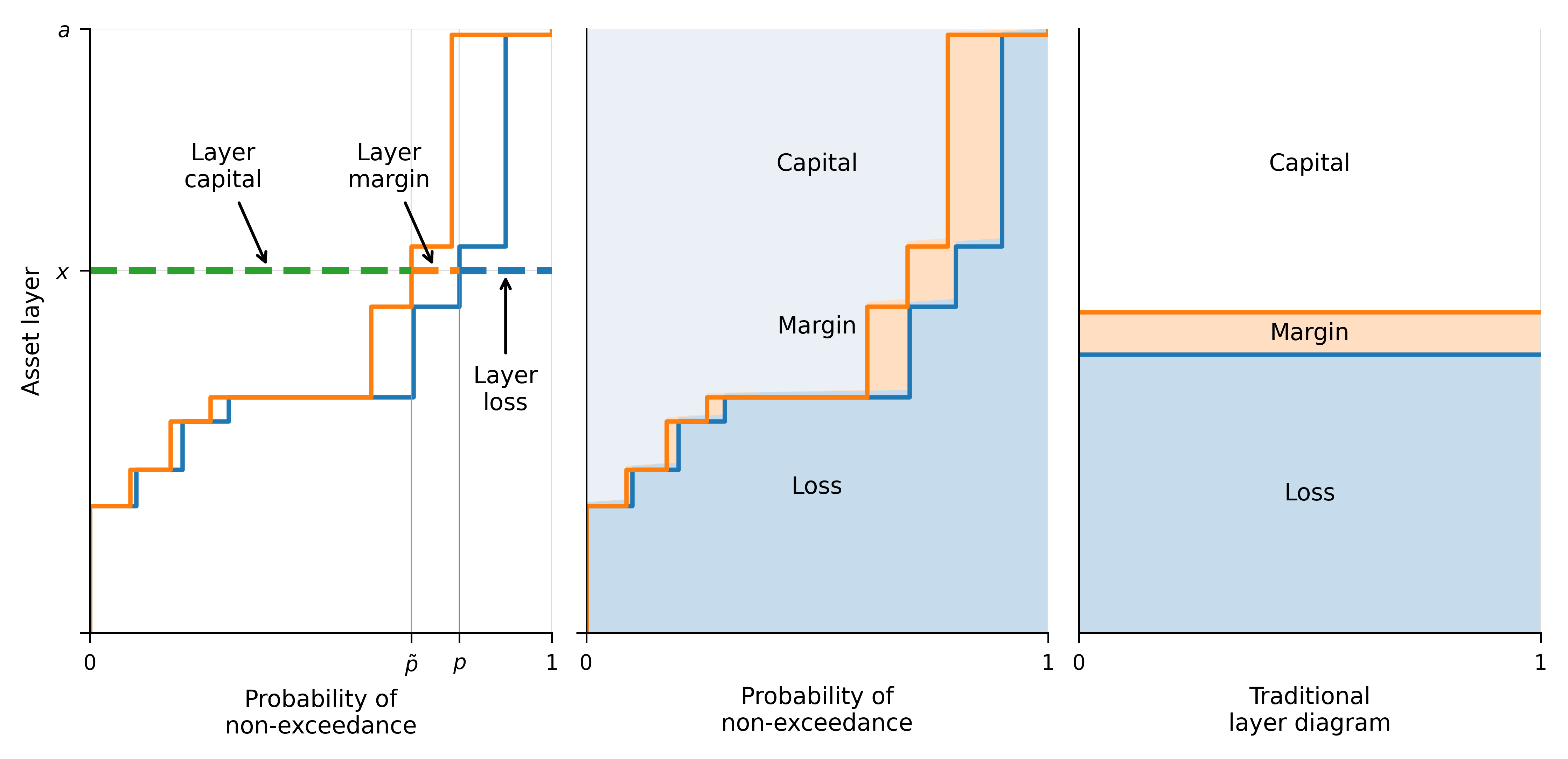
Let’s look more closely at Equation 4.5. From our setup, the largest possible loss and \(\sum \Delta X_k=a\). Using that, recall the two ways of computing the mean (integration by parts): \[ \mathsf E[X]=\sum_{k=0}^{n} X_k p_k = \sum_{k=0}^{n-1} \Delta X_k S_k. \] The right-hand term is a sum over expected losses in each layer \(k\). This formula is illustrated in Figure 4.2 by the blue area and explained in the context of the Lee diagram in chapter 3 of Mildenhall and Major (2022). Now, if each layer of capital costs \(g(S_j)\), we can use integration by parts to get \[ \begin{aligned} P &= \sum_{k=0}^{n-1} g(S_k) \Delta X_k \\ &= \sum_{k=0}^{n-1} g(S(X_k))(X_{k+1} - X_k) \\ &= \sum_{k=0}^{n} (g(S_{k-1}) - g(S_{k})))X_k \\ &= \sum_{k=0}^{n} q_k X_k \end{aligned} \tag{4.6}\] where \(g(S_{-1}):=1\). Refer to Figure 4.2. The size of each vertical step is \(\Delta X_k\), and the left-to-right distance from each blue (respectively, orange) vertical step to the \(p=1\) axis is \(S_k\) (respectively, \(g(S_k)\)). The area under the blue line is the expected loss. The area under the orange line is the premium, corresponding to either expression in Equation 4.6. The difference is the margin, shown in orange shading in the second panel. The complement of premium is capital, above the orange line, shaded in light blue. This view of the relationship between capital, margin, and loss is dramatically different from the conventional view in the third panel.
In Equation 4.6, the last two formulas can be interpreted as the expected value outcomes \(X_k\) with respect to adjusted or distorted probabilities \(q_k\), analogous to \(p_k = S_{k-1} - S_k\). (This symbol \(q\) for a probability measure is not to be confused with capital amount \(Q\) symbol.) Notice that \(\sum_{j=0}^{n} q_j = 1\). Since all \(q_j\) are nonnegative, collectively they satisfy the properties of a probability distribution.
Exercise. For \(\mathsf E[X]\), prove that \(\sum_j S_j \Delta X_j = \sum_j p_j X_j\).
Solution. \[ \begin{aligned} \sum_{j=0}^n p_j X_j &= \sum_{j=1}^n (S_{j-1}-S_j) X_j \\ &= \sum_{j=0}^{n-1} S_j X_{j+1} - \sum_{j=1}^n S_j X_j \\ &= \sum_{j=0}^{n-1} S_j \Delta X_{j} \end{aligned} \] because \(S_0 X_0 = S_n X_n = 0\).
Exercise. For \(\rho(X)\), prove that \(\sum_j g(S_j) \Delta X_j = \sum_j q_j X_j\).
Solution. This is essentially the same derivation as for \(\mathsf E[X]\) but with \(g(S)\) substituted for \(S\) and \(q\) substituted for \(p\).
We can go one step further and write \[ P = \sum_{k=0}^{n} q_kX_k = \sum_{k=0}^{n} X_k Z_k p_k. \tag{4.7}\] The likelihood ratios \(Z_j=q_j/p_j\) individually can be less than, equal to, or greater than one, but their expected value equals one.
Recall that for our example \(\iota=0.15\), \(\nu=0.86956\), and \(\delta=0.13043\). Table 4.4 tabulates the portfolio expected loss and premium based on the CCoC distortion which we define in Section 4.6. We can see, comparing to Table 4.11, that the same portfolio premium is obtained.
| \(k\) | \(p\) | Portfolio \(X_k\) | Layer size \(\Delta X_k\) | Exceedance Pr \(S_k\) | Distorted \(g(S)\) | \(S\Delta X\) | \(g(S)\Delta X\) |
|---|---|---|---|---|---|---|---|
| 0 | 0 | 0 | 22 | 1 | 1 | 22 | 22 |
| 1 | 0.1 | 22 | 6 | 0.9 | 0.913 | 5.4 | 5.478 |
| 2 | 0.1 | 28 | 8 | 0.8 | 0.826 | 6.4 | 6.609 |
| 3 | 0.1 | 36 | 4 | 0.7 | 0.739 | 2.800 | 2.957 |
| 4 | 0.4 | 40 | 15 | 0.3 | 0.391 | 4.500 | 5.870 |
| 5 | 0.1 | 55 | 10 | 0.2 | 0.304 | 2 | 3.043 |
| 6 | 0.1 | 65 | 35 | 0.1 | 0.217 | 3.5 | 7.609 |
| 7 | 0.1 | 100 | 0 | 0 | 0 | 0 | 0 |
| Sum | 1 | 100 | 46.6 | 53.565 |
4.5 Pricing units via pricing layers
A portfolio’s premium, computed by an SRM, has an NA to units.
We are now in a position to consider the pricing of portfolio units. Let the portfolio aggregate loss be the sum of \(m\) unit losses: \[ X = \sum_{i=1}^m X^i. \] The various \(X^i\) may or may not be correlated. We assume they are nonnegative.
It is natural to look at Equation 4.6 and suppose that the price of \(X^i\) should be \[ P^i = \sum_{j=0}^a q_j X_j^i. \tag{4.8}\] Note the resemblance of this to the expected value of \(X^i\): \[ L^i = \sum_{j=0}^a p_j X_j^i. \tag{4.9}\] Finally, of course, unit margin (analogous to Equation 4.1) is simply the difference: \[ M^i = P^i-L^i. \tag{4.10}\]
This decomposition of \(P\) into \(\sum_i P^i\) is known as the NA of an SRM—so-called because it relies on no additional assumptions. It is the distorted expectation of \(X^i\). Other ways of writing it are \[ P^i =\ E[Z\cdot X^i] = \mathsf E[X^i]\mathsf E[Z] + \mathsf{cov}(Z,X^i) = \mathsf E[X^i] + \mathsf{cov}(Z,X^i) \tag{4.11}\] because \(\mathsf E[Z]=1\). The first expression resembles a pricing kernel in modern finance theory or a co-measure (Venter et al. 2006). The last expression resembles the Capital Asset Pricing Model.
Exercise. Verify Equation 4.11.
Solution. \(\mathsf{cov}(Z,X)=\mathsf E[ZX] - \mathsf E[Z]\mathsf E[X]=\mathsf E[ZX] -\mathsf E[X]\) because \(\mathsf E[Z]=1\).
Why do we require unique outcome values for \(X\)? To enforce a unique ordering of outcomes. The values \(q_k\) depend on the order of events. If there are multiple \(k\) with equal \(X_k\), that ambiguity doesn’t matter for computing total premium \(P\). But when we consider allocations to units it does, because it allows some unwanted flexibility in \(q_k\). When the outcomes of \(X\) are distinct we are also guaranteed that the NA equals the marginal cost of increasing business in unit \(i\). Since the outcomes are distinct, the order of outcomes of \(X\) and of \(X+\epsilon X^i\) is the same provided \(\epsilon\) is small enough (positive or negative). As noted above, \(q\) reproduces stand-alone pricing for all risks comonotonic with (same order as) \(X\). Thus \[ \begin{aligned} \nabla^i \rho_X &= \lim_{\epsilon\to 0}\frac{\rho(X + \epsilon X^i) - \rho(X)}{\epsilon} \\ &= \lim_{\epsilon\to 0}\frac{\mathsf E_q[X + \epsilon X^i] - \mathsf E_q[X]}{\epsilon} \\ &= \lim_{\epsilon\to 0}\frac{\mathsf E_q[X] + \mathsf E_q[\epsilon X^i] - \mathsf E_q[X]}{\epsilon} \\ &= \lim_{\epsilon\to 0}\frac{\epsilon \mathsf E_q[X^i]}{\epsilon} \\ &= \mathsf E_q[X^i]. \end{aligned} \] This very important result was proved by Delbaen around 2000. It shows that the NA is the natural extension of Tasche (1999).
4.6 Five representative distortion functions
We now introduce five carefully selected families of distortion functions: constant cost of capital (CCoC), proportional hazards (PH), Wang transform, dual moment transform, and TVaR. Table 4.5 shows the formulas for each and parameters selected to achieve InsCo’s portfolio pricing consistent with an expected return of \(\iota=0.15\). For the Wang distortion, introduced in Wang (2000), \(\Phi\) is the standard Gaussian cumulative distribution function. For the PH (respectively, other four) a lower (respectively, higher) parameter indicates a more risk averse distortion resulting in higher prices for a given risk.
| Distortion | Formula | Parameter |
|---|---|---|
| CCoC | \(\nu s+\delta\) | \(\iota=0.1500\) |
| PH | \(s^\alpha\) | \(\alpha=0.3427\) |
| Wang | \(\Phi(\Phi^{-1}(s)+\lambda)\) | \(\lambda=0.7205\) |
| Dual | \(1-(1-s)^m\) | \(m=1.5951\) |
| TVaR | \(1\wedge s/(1-p)\) | \(p=0.2713\) |
Figure 4.3 plots the five distortion functions and distorted probabilities. The blue star above \(s=0\) on the right reminds us of the probability mass for the CCoC . The thin black line shows the reference \(Z=1\) line, where risk-adjusted and objective probabilities are equal. The plots explain the order of the distortions: CCoC gives the greatest weight to the worst \(s=0\) loss (remember the \(*\) above the worst event) and TVaR the least. Conversely, TVaR gives the greatest weight to moderate losses between the 25th and 75th percentiles. Table 4.6 shows the \(g(s)\) values corresponding to each of the five distortions for \(S\) values in our example, Table 4.7 shows the distorted probabilities (\(q\)) associated with each distortion function, and Table 4.8 shows the \(Z=q/p\) factor for each distortion, showing the proportionate increase or decrease over objective probabilities \(p\).

| \(k\) | \(S\) | CCoC | PH | Wang | Dual | TVaR |
|---|---|---|---|---|---|---|
| 0 | 1 | 1 | 1 | 1 | 1 | 1 |
| 1 | 0.9 | 0.9130 | 0.9269 | 0.9478 | 0.9746 | 1 |
| 2 | 0.8 | 0.8261 | 0.8515 | 0.8819 | 0.9233 | 1 |
| 3 | 0.7 | 0.7391 | 0.7734 | 0.8071 | 0.8535 | 0.9606 |
| 4 | 0.3 | 0.3913 | 0.4200 | 0.4279 | 0.4339 | 0.4117 |
| 5 | 0.2 | 0.3043 | 0.3136 | 0.3089 | 0.2995 | 0.2745 |
| 6 | 0.1 | 0.2174 | 0.1903 | 0.1739 | 0.1547 | 0.1372 |
| 7 | 0 | 0 | 0 | 0 | 0 | 0 |
| \(k\) | \(p\) | CCoC | PH | Wang | Dual | TVaR |
|---|---|---|---|---|---|---|
| 1 | 0.1 | 0.0870 | 0.0731 | 0.0522 | 0.0254 | 0 |
| 2 | 0.1 | 0.0870 | 0.0754 | 0.0660 | 0.0513 | 0 |
| 3 | 0.1 | 0.0870 | 0.0781 | 0.0748 | 0.0698 | 0.0394 |
| 4 | 0.4 | 0.3478 | 0.3534 | 0.3791 | 0.4196 | 0.5489 |
| 5 | 0.1 | 0.0870 | 0.1064 | 0.1190 | 0.1344 | 0.1372 |
| 6 | 0.1 | 0.0870 | 0.1233 | 0.1350 | 0.1448 | 0.1372 |
| 7 | 0.1 | 0.2174 | 0.1903 | 0.1739 | 0.1547 | 0.1372 |
| \(k\) | \(p\) | CCoC | PH | Wang | Dual | TVaR |
|---|---|---|---|---|---|---|
| 1 | 1 | 0.8696 | 0.7310 | 0.5216 | 0.2540 | 0 |
| 2 | 1 | 0.8696 | 0.7541 | 0.6598 | 0.5134 | 0 |
| 3 | 1 | 0.8696 | 0.7810 | 0.7480 | 0.6979 | 0.3941 |
| 4 | 1 | 0.8696 | 0.8834 | 0.9479 | 1.0490 | 1.3723 |
| 5 | 1 | 0.8696 | 1.0640 | 1.1899 | 1.3439 | 1.3723 |
| 6 | 1 | 0.8696 | 1.2329 | 1.3502 | 1.4479 | 1.3723 |
| 7 | 1 | 2.1739 | 1.9033 | 1.7391 | 1.5470 | 1.3723 |
All of the distortions underweight events 1 through 3. Event 4 has the median loss. TVaR, while assigning zero weight to the lowest losses, is still the most body focused because it overweights events 4 and above—equally—and among all distortions applies the smallest weight to the largest loss. CCoC, however, applies the largest weight to event 7 (the largest loss) and only that event. The other distortions apply weights to event 7 in the order of presentation in the table. The ordering for event 4, representing body focus, is the opposite of the ordering for event 7, representing tail focus.
The results obtained by using the Wang distortion are shown in Table 4.9.
| \(k\) | \(p\) | Unit A \(X^1_k\) | Unit B \(X^2_k\) | Unit C \(X^3_k\) | Portfolio \(X_k\) | \(S\) | \(g(S)\) | \(q\) | \(Z\) |
|---|---|---|---|---|---|---|---|---|---|
| 0 | 0 | 0 | 0 | 0 | 0 | 1 | 1 | 0 | 0 |
| 1 | 0.1 | 15 | 7 | 0 | 22 | 0.9 | 0.948 | 0.052 | 0.522 |
| 2 | 0.1 | 15 | 13 | 0 | 28 | 0.8 | 0.882 | 0.066 | 0.660 |
| 3 | 0.1 | 5 | 20 | 11 | 36 | 0.7 | 0.807 | 0.075 | 0.748 |
| 4 | 0.4 | 10 | 24 | 6 | 40 | 0.3 | 0.428 | 0.379 | 0.948 |
| 5 | 0.1 | 26 | 19 | 10 | 55 | 0.2 | 0.309 | 0.119 | 1.190 |
| 6 | 0.1 | 17 | 8 | 40 | 65 | 0.1 | 0.174 | 0.135 | 1.350 |
| 7 | 0.1 | 16 | 20 | 64 | 100 | 0 | 0 | 0.174 | 1.739 |
| \(L=\mathsf E_p\) | 13.4 | 18.3 | 14.9 | 46.6 | |||||
| \(P=\mathsf E_q\) | 14.109 | 18.637 | 20.818 | 53.565 | |||||
| \(M=P-L\) | 0.709 | 0.337 | 5.918 | 6.965 | |||||
| Prop of tot \(M\) | 0.102 | 0.048 | 0.850 | 1 |
So far, we have seen how to allocate premium \(P\) (and therefore margin \(M\), via Equation 4.1) to portfolio units via the NA of an SRM, once a distortion function \(g(s)\) is available. Chapter 8 discusses how to choose a distortion function. A premium allocation allows us to compute economic value added by unit, the actual premium in excess of required premium, and to assess static portfolio performance by unit—motivations for performing capital allocation in the first place (Chapter 5). In many ways it is also a good place to stop.
However, if desired, the ideas behind the natural premium allocation can be extended to give a capital allocation consistent with SRM premium allocation. This is discussed in Section 8.3.
4.7 The Industry Standard Approach and its problems
In this section we step back to the 1990s, before the layer approach was formally introduced, and describe how what we call the Industry Standard Approach (ISA) evolved and the problems it generates. At that time, actuaries determined prices on a stand-alone basis, because in an efficient market prices are additive. They used the formula premium equals loss cost plus margin, and margin was computed as cost of capital times amount of capital, giving (Table 4.1 P1, P3a): \[ P = L + \iota Q = \nu L + \delta a. \tag{4.12}\] It was deemed obvious that the cost of capital should vary by unit according to different levels of systematic risk. However, attempts to compute underwriting betas from accounting data failed or had standard errors that swamped differences by unit. In consequence, it became standard to assume that \(\iota\) was constant across units. This story emerges in Myers and Cohn (1987), Cummins (2000), and Kozik (1994).
Around the same time, Tasche (1999) pointed out that marginal capital is the “only definition for the risk contributions which is suitable for performance measurement.” Tasche’s analysis relies on a constant cost of capital to equate needs more capital with needs more margin. That relationship obviously fails if capital costs vary. As a result, by 2000, the ISA was to use a CCoC and marginal capital by unit to steer portfolios. This is called RAROC, return on risk adjusted capital: the return is constant but the capital varies with risk.
As we saw in Section 4.4, in the mid-1990s Wang and others introduced the idea of pricing by layer. It is easy to translate Equation 4.12 into the layer framework. Without loss of generality, we can assume the four adjustments of Section 4.3, so \(a=\max(X)\). Then, \[ \begin{aligned} P &= L + \iota Q \\ &= \nu\, L + \delta \, a \\ &= \nu\, \mathsf E[X] + \delta \, \max(X) \\ &= \nu \sum_{k=0}^{n-1} S_k\Delta X_k + \delta \sum_{k=0}^{n-1} \Delta X_k \\ &= \sum_{k=0}^{n-1} (\nu S_k + \delta) \Delta X_k \\ &= \sum_{k=0}^{n-1} g(S_k) \Delta X_k \end{aligned} \] is exactly the premium associated with the CCoC distortion \(g(s)=\nu s + \delta\). Here an important transformation has occurred. ISA (reasonably) assumed a CCoC by unit. The layer view shows that constant unit costs mathematically imply a CCoC by layer, an implication that went unremarked at the time. The problem is that capital costs are manifestly not constant by layer. Numerous websites such as the Federal Reserve’s FRED and Bank of America’s ICE provide the latest information on credit yield spreads. Low-risk instruments such as government or AAA-rated bonds require lower yields than non-investment-grade or junk bonds. This is true even after corrections are made to the yield calculations to take default probability into account (Heynderickx et al. 2016).

Aside from the factual inconvenience of making an empirically false assumption, the CCoC distortion causes other problems. It is numerically unstable because it puts a large weight on the worst outcome and underweights all others. For the same reason, it is very averse to tail risk but blithely ignores volatility risk around the mean. None of the four other distortions in Table 4.5 has these problems: all have a cost of capital that varies by layer and distribute their probability weight more evenly across events. CCoC is further unusual because it provides no diversification benefit for independent risks.
Exercise. Show that CCoC distortion pricing is additive for independent risks.
Solution. \(P=\nu \mathsf E[X] + \delta\max(X)\) and expectation and maximum are additive for independent risks.
Table 4.10 shows the calculation of \(q_k\), \(\mathsf E[X]\), and the price of \(X\) using the \(q\,\)s. It gives the same result as Table 4.4.
| \(k\) | \(p\) | Portfolio \(X_k\) | Layer size \(\Delta X_k\) | Exceedance Pr \(S_k\) | \(pX\) | Distorted \(q\) | \(qX\) | \(Z=q/p\) |
|---|---|---|---|---|---|---|---|---|
| 0 | 0 | 0 | 22 | 1 | 0 | 0 | 0 | |
| 1 | 0.1 | 22 | 6 | 0.9 | 2.2 | 0.087 | 1.913 | 0.870 |
| 2 | 0.1 | 28 | 8 | 0.8 | 2.800 | 0.087 | 2.435 | 0.870 |
| 3 | 0.1 | 36 | 4 | 0.7 | 3.6 | 0.087 | 3.130 | 0.870 |
| 4 | 0.4 | 40 | 15 | 0.3 | 16 | 0.348 | 13.913 | 0.870 |
| 5 | 0.1 | 55 | 10 | 0.2 | 5.5 | 0.087 | 4.783 | 0.870 |
| 6 | 0.1 | 65 | 35 | 0.1 | 6.5 | 0.087 | 5.652 | 0.870 |
| 7 | 0.1 | 100 | 0 | 0 | 10 | 0.217 | 21.739 | 2.174 |
| Sum | 1 | 100 | 53.565 |
Let us examine the allocations obtained by the CCoC assumption and compare the results obtained by using the Wang distortion.
The \(Z\) values associated with the Wang distortion are shown in Table 4.9; the CCoC values are in Table 4.10. The last three \(Z\) values are greater than one for Wang, whereas only the last one is greater than one for CCoC.
| Variable | Unit A \(X^1_j\) | Unit B \(X^2_j\) | Unit C \(X^3_j\) | Total \(X_j\) |
|---|---|---|---|---|
| \(L=\mathsf E[X]\) | 13.4 | 18.3 | 14.9 | 46.6 |
| \(a=\mathsf{TVaR}\) | 16 | 20 | 64 | 100 |
| \(Q=\nu\mathsf{XTVaR}\) | 2.261 | 1.478 | 42.696 | 46.435 |
| \(P\) | 13.739 | 18.522 | 21.304 | 53.565 |
| \(M=P-L\) | 0.339 | 0.222 | 6.404 | 6.965 |
| Allocation of \(M\) | 0.049 | 0.032 | 0.919 | 1 |
| \(\iota=M/Q\) | 0.150 | 0.150 | 0.150 | 0.150 |
For InsCo, the results of the CCoC allocation are shown in Table 4.11. Unit C, because of its outsize presence in the worst event, gets 91.9% of the capital and margin allocated to it. This tends to be the outcome from practical applications of the standard approach: the thick-tail lines of business get nearly all the capital and margin allocated to them and the thin tail lines get a free pass. With the Wang distortion, instead of getting 8% of the margin, Units A and B get 15% of the margin.
To recap: It is often assumed that one can transition from allocating capital to allocating cost of capital (i.e., margin or premium) simply by multiplying capital by a single cost of capital rate. Indeed, it is basically that simple when dealing with the entire business portfolio in aggregate (because the total cost of capital is the weighted average cost times the amount). However, when disaggregating results into units this simple tactic founders for two reasons. First, as we saw above, purported capital allocation procedures based on marginal analysis of the capital risk measure aren’t really relevant to pricing. Second, it is likely that CCoC is not appropriate because there is no single cost of capital rate that applies to all layers of risk and different units consume a different mix of capital by layer. Each contributor to the business has its own risk profile and its own joint dependency with the aggregate risk profile—and therefore its own cost of capital.
Understanding the flaws of the ISA highlights the improvements offered by layer pricing and allocation. First, by choice of distortion \(g\), we can match the cost of capital by layer to market observables. Second, since unit consumption of capital varies by layer, the calculation naturally produces different returns by unit in total, thus solving the problem from the 1990s originally tackled using underwriting betas. Moreover, the solution is consistent with the observations in Table 1.1. Thick-tailed, catastrophe exposed lines consume relatively more higher layer capital. Higher layer capital is less exposed to loss (like a higher rated bond) and earns a lower return. Thus, such lines will be charged with a lower cost of capital. They will run with lower leverage too, resulting in a low loss ratio. This is why catastrophe reinsurance works economically: it substitutes expensive equity for cheaper debt-like capital.
4.8 Pricing events: An explanation
We saw in Equation 4.6 that premium can be computed as the expected value of the loss outcomes \(X_k\) with respect to altered probabilities \(q_k\). This seems to provide us with an interpretation of pricing events, rather than layers, but that interpretation comes with a big caveat.
So far, this is just algebra. We would like to interpret \(Z_k\) as the unique state price for event \(k\) and take this as the definitive statement of event pricing, backed by a no-arbitrage argument. Alas, that interpretation is not quite correct for reasons that involve bid-ask spreads and are beyond the scope of this monograph. They are explained more fully in chapter 10 of Mildenhall and Major (2022).
However, it does provide a set of internally consistent allocations to events as part of the total. The portfolio premium \(P\) can be regarded as an expectation taken under the new, \(q\) probability \(\mathsf E_q[X]\) or, equivalently, as a weighted expectation \(\mathsf E_p[ZX]\) under the original distribution with \(Z\) as the weight. Using the \(q\) probabilities this way is also applying an SRM to \(X\), equivalent to how we did it previously through layer pricing. Using a distorted expectation to represent price is very much in the spirit of using risk neutral probabilities in modern finance; they are not always unique there, either. Thus, if we fix \(X\), then we can price any subunit \(X^i\) of \(X\) using \(q_k\) \[ \text{allocation to\ } X^i = \sum_k X^i_k q_k \] and never never run into logical or economic inconsistencies. This is exactly the same as the procedure for computing coTVaR and is the basis of the NA.
In general, Equation 4.7 can also be used to price any set of outcomes \(Y_k\) that are comonotonic with \(X_k\)—in the sense that it will give the same stand-alone price as the spectral measure. This follows because the ordering of events determined by \(X_k\) gives a nondecreasing ordering of events for \(Y_k\). (The converse may not be true. For example \(Y_k=c\) is constant is comonotonic with \(X_k\), but would admit any ordering of events as nondecreasing.) In our case, each layer is comonotonic with the total, so Equation 4.7 can be seen as an application. In general, the allocation will be less than or equal to the stand-alone price. There is a lower bound too, see chapter 10 of Mildenhall and Major (2022).
4.9 Summary
Spectral pricing gives the price of the total (whole portfolio) risk in the market. In contrast, the NA gives an allocation to part of the total risk—and crucially depends on the total. The allocation equals the stand-alone spectral price only in the case that the risk is comonotonic with the total risk. You can use and interpret the NA as a risk-adjusted expected value, and never have a problem, provided you understand it in the context of a total \(X\). As an allocation, it has the beauty of being consistent with a marginal approach in the case that all the outcomes of \(X\) are distinct. In fact, it is consistent if and only if all the outcomes are distinct.
Spectral prices are sub-additive, so insureds benefit from pooling together—providing a motivation for insurance companies to exist! The insurer has to figure out how to allocate that lower price fairly among its insureds. Of course, the insurer is happy with any price greater than equal to a fair allocation, particularly with the marginal interpretation of allocation. The marginal interpretation drives profit maximizing behavior in a standard sense.
We conceptualized the cash flows between policyholders and investors via the InsCo one-year model with claim payouts \(X\) and probabilities \(p\). We distinguished between capital and pricing risk measures. Portfolio funding was subject to the constraints \(P+Q=a\) and \(P=L+M\) with the investor return being \(\iota=M/Q\), resulting in Equation 4.2: \[ P = L + \delta (a-L) = L + \iota Q. \]
These relationships were carried down to hold for each asset layer. Pricing was done via SRMs through distorted probabilities with \(S\) being replaced by \(g(S)\) and \(p\) being replaced by \(q=\Delta g(S)\). This allows us to price any cash flow that is a function of specific value outcomes \(X\). In particular we can price the units of the portfolio: lines of business or even policies.
We saw that while understanding the marginal impact of increasing a unit’s exposure on the overall asset requirement (the capital measure) was meaningful for risk management, it had little relevance to pricing per se. We also saw that assuming a CCoC had troublesome implications about event weights \(Z=q/p\).
4.10 Algorithms
The next two algorithms are taken from Mildenhall and Major (2022). They are included here for completeness and ease of reference. As is often the case, they look more intimidating than they are—build the spreadsheet and you’ll see they are quite straightforward!
4.10.1 Algorithm to evaluate an SRM on a discrete random variable
Algorithm Input: \(X\) is a discrete random variable, taking values \(X_j\ge 0\), and \(p_j=\mathsf P(X=X_j)\), \(j=1,\dots, n\). \(\rho_g\) is an SRM.
Follow these steps to determine \(\rho_g(X)\).
Algorithm Steps
- Pad the input by adding a zero outcome \(X_0=0\) with probability 0.
- Sort events by outcome \(X_j\) into ascending order.
- Group by \(X_j\) and sum the corresponding \(p_j\). Relabel events \(X_0 < X_1 < \dots < X_{n'}\) and probabilities \(p_0,\dots, p_{n'}\). All \(X_j\) are distinct.
- Decumulate probabilities to determine the survival function \(S_j:=S(X_j)\) using \(S_0=1-p_0\) and \(S_j=S_{j-1}-p_j\), \(j>0\).
- Distort the survival function, computing \(g(S_j)\).
- Difference \(g(S_j)\) to compute risk-adjusted probabilities \(\Delta g(S_0)=1-g(S_0)\), \(\Delta g(S_j)=g(S_{j-1})-g(S_j)\), \(j > 0\).
- Sum-Product to compute \(\rho_g(X)= \sum_j X_j\,\Delta g(S_j)\).
Steps (4) and (6) are inverse to one another. The transition \(p\to S\to gS \to \Delta gS\) from input probabilities to risk-adjusted probabilities is used in all SRM-related algorithms.
The algorithm computes the outcome-probability formula \[\begin{equation*} \rho_g(X) = \int_0^\infty xg'(S(x))\,dF(x) = \sum_{j>0} X_j \Delta g(S_j). \end{equation*}\] When \(X\) is discrete the Steiltjes integral becomes a sum—the joy of using \(dF\). We can also use the survival function form with \(\Delta X_j=X_{j+1}-X_j\) \[\begin{equation*} \rho_g(X) = \int_0^\infty g(S(x))\,dx = \sum_{j\ge 0} g(S_j) \Delta X_j. \end{equation*}\]
4.10.2 Algorithm to compute the linear NA for discrete random variables
Algorithm Inputs:
- The outcome values \((X^1_j,\dots,X^m_j)\), \(j=1,\dots, n\), of a discrete \(m\)-dimensional multivariate loss random variable. Outcome \(j\) occurs with probability \(p_j\). \(X_j=\sum_i X^i_j\) denotes the total loss for outcome \(j\).
- An SRM \(\rho_g\) associated with the distortion function \(g\).
Follow these steps to determine \(D^n\rho_X(X^i)\), the NA of \(\rho(X)\) to unit \(i\).
Algorithm Steps
- Pad the input by adding a zero outcome \(X^1_0=\cdots=X^m_0=X_0=0\) with probability \(p_0=0\).
- Sort events by total outcome \(X_j\) into ascending order.
- Group by \(X_j\) and take \(p\)-weighted averages of the \(X^i_j\) within each \(i\) and \(X_j=x\) group. Sum the corresponding \(p_j\). Relabel events using \(j=0,1,\dots, n'\) as \(X^i_j\) and probabilities \(p_0,\dots, p_{n'}\).
- Decumulate probabilities to determine the survival function \(S_j:=S(X_j)\) using \(S_0=1-p_0\) and \(S_j=S_{j-1}-p_j\), \(j>0\).
- Distort the survival function, computing \(g(S_j)\).
- Difference \(g(S_j)\) to compute risk-adjusted probabilities \(\Delta g(S_0)=1-g(S_0)\) and \(\Delta g(S_j)=g(S_{j-1})-g(S_j)\), \(j > 0\).
- Sum-Product to compute \(\rho_g(X)= \sum_j X_j\,\Delta g(S_j)\) and \[\begin{equation}\label{eq:Dn-rho-xi} D^{n}\rho_X(X_i) = \mathsf E[X_iZ] = \sum_j X^i_j\,Z_j\,p_j = \sum_j X^i_j\,\frac{\Delta g(S_j)}{p_j}\,p_j = \sum_j X^i_j\,\Delta g(S_j). \end{equation}\]
Comments.
- When the data are produced by a simulation model, \(n\) equals the number of events and \(m\) the number of units. With realistic data, \(n\) is in the range thousands to millions, and \(m\) ranges from a handful up to the hundreds for a full corporate model.
- Step (1) only results in a new outcome row when the smallest \(X_j\) observation is \(>0\).
- The averages in Step 3 are implemented as \[\begin{equation} \label{eq:EXiX-discrete-simple} \kappa^i(x) = \mathsf E[X_i\mid X=x] = \frac{\sum_{j:X_j = x} p_j\,X^i_j} {\sum_{j:X_j = x}p_j}. \end{equation}\]
- After Step (3), the \(X_j\) are distinct, they are in ascending order, \(X_0=0\), and \(p_j=\mathsf P(X=X_j)\).
- The backward difference \(\Delta g(S_j)\) computed in Step (6) replaces \(g'(S)dF(x)\) in various formulas.
- is an exact equation for a discrete distribution. Approximation occurs if it is applied to the empirical distribution of a discrete sample representing a different underlying distribution, possibly one with density.