This chapter reproduces many of the exhibits from the main text using Python and the aggregate package. It also describes how to extend to more realistic examples. Throughout, we have included only terse subsets of code so the reader can focus on the results and the output. Instructions for obtaining the full code are provided below.
9.1Aggregate and Python
aggregate is a Python package that can be used to build approximations to compound (aggregate) probability distributions quickly and accurately, and to solve insurance, risk management, and actuarial problems using realistic models that reflect underlying frequency and severity. It delivers the speed and accuracy of parametric distributions to situations that usually require simulation, making it as easy to work with an aggregate (compound) probability distribution as the lognormal. aggregate includes an expressive language called DecL to describe aggregate distributions.
The aggregate package is available on PyPi, the source code is on GitHub at https://github.com/mynl/aggregate, and there is extensive documentation. The Aggregate class and DecL lanaguage are described in Mildenhall (2024). There is also an extensive series of videos introducing various capabilities available on YouTube.
9.2Aggregate and R
Python packages can be used in R via the reticulate library. Python and R code can also be mixed in RMarkdown (now Quarto) files. This short video explains how to use aggregate from R.
9.3 Reproducing the code examples
To reproduce the Python code examples, you must set up your environment and then install aggregate using
pip install aggregate
The formatting of the examples relies on greater_tables, which can be installed in the same way. The installation process will also install several standard packages, such as numpy and pandas, that it depends on. If you get an error message about other missing packages, you can install them with pip. All the code in the monograph runs on aggregate version 0.24.0 and should run on any later version. If you have an older version installed, you can updated it with pip install -U aggregate.
Once aggregate is installed, start by importing basic libraries. The next code block shows the relevant aggregate function. The class GT from greater_tables is used to format DataFrames consistently.
from aggregate import ( Portfolio, # creates multi-unit portfolios make_ceder_netter, # models reinsurance Distortion # creates a Distortion function)from greater_tables import GT # consistent table format
Online resources. Complete code samples can be extracted from the online version of the monograph, available at https://cmm.mynl.com/. Each code block has a small copy icon in the upper right-hand corner. The code blocks on each page can all be shown or hidden using the </>Code control at the top of the page. To download the original qmd file, use the View Source option under the same control. Alternatively, the entire Quarto (previously RMarkdown) source can be downloaded from GitHub at https://github.com/mynl/CapitalModeling (CAS TO INSERT OWN LINK).
9.4 Reproducing the discrete example
9.4.1 Input data and setup
The InsCo example running through this monograph is based on the 10 events shown in Table 9.1, which reproduces Table 2.1, and adds the mean and CV. For reference, here is the code to create the underlying dataframe.
Table 9.1: The 10 equally likely simulations underlying the basic examples.
index
A
B
C
Total
0
5
20
11
72
1
7
33
0
80
2
15
13
0
56
3
15
7
0
44
4
13
20
7
80
5
5
27
8
80
6
15
16
9
80
7
26
19
10
110
8
17
8
40
130
9
16
20
64
200
EX
13.4
18.3
14.9
93.2
CV
0.453
0.412
1.324
0.455
Now we create an aggregatePortfolio class instance based on the loss_sample simulation output. The next block shows how to do this, using the Portfolio.create_from_sample method. TMA1 is a label, and loss_sample is the dataframe created previously. The other arguments specify working with unit-sized buckets bs=1 appropriate for our integer losses and to use \(256=2^8\) buckets, log2=8.
The next line of code displays Table 9.2, which shows summary output from the object wport by accessing its describe attribute. The summary includes the mean, CV, and skewness. The model and estimated (Est) columns are identical because we specified the distribution directly; no simulation or Fast Fourier Transform-based numerical methods are employed.
Table 9.2: Summary statistics for the base example.
unit
X
E[X]
Est E[X]
CV(X)
Est CV(X)
Skew(X)
Est Skew(X)
A
Freq
1
0
Sev
13.4
13.4
0.453
0.453
0.281
0.281
Agg
13.4
13.4
0.453
0.453
0.281
0.281
B
Freq
1
0
Sev
18.300
18.300
0.412
0.412
0.269
0.269
Agg
18.300
18.300
0.412
0.412
0.269
0.269
C
Freq
1
0
Sev
14.9
14.900
1.324
1.324
1.603
1.603
Agg
14.9
14.900
1.324
1.324
1.603
1.603
total
Freq
3
0
Sev
15.533
15.533
0.827
1.884
Agg
46.6
46.600
0.471
0.471
1.177
1.177
Next, we need to calibrate distortion functions to achieve the desired pricing. The example uses full capitalization throughout (assets equal the maximum loss), which is equivalent to a 100% percentile level (see Table 9.5) and assumes the cost of capital is 15%. The code runs the calibration by calling wport.calibrate_distortions with arguments for the capital percentile level Ps and cost of capital COCs. The arguments are passed as lists because the routine can be used to solve for several percentile levels and costs simultaneously. Table 9.3 shows the resulting parameters, which match those in Table 4.5.
Code
# calibrate to 15% return at p=100% capital standardwport.calibrate_distortions(Ps=[1], COCs=[.15]);
Table 9.3: Distortion functions calibrated to 15% return on full capital.
method
P
param
error
ccoc
53.565
0.150
0
ph
53.565
0.720
0.000
wang
53.565
0.343
0.000
dual
53.565
1.595
-0.000
tvar
53.565
0.271
0.000
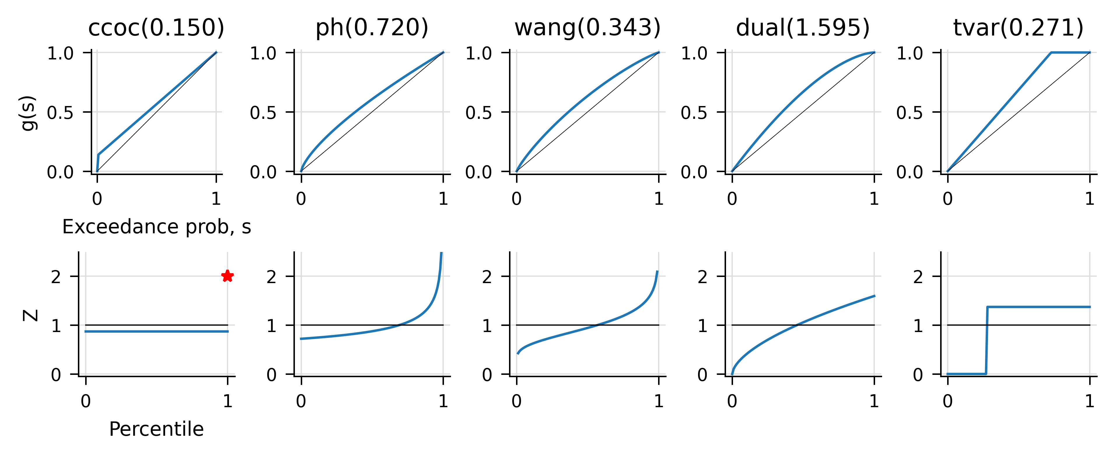
Figure 9.1 shows the resulting distortion \(g\) functions (top) and the probability adjustment \(Z=q/p\) (bottom). The red star indicates a probability mass at \(p=1\).
Figure 9.1: Distortion functions (top row) and distortion probability adjustment functions (bottom row).
For technical reasons (discussed in Section 4.3 as well as chapter 14.1.5 in Mildenhall and Major (2022), see especially Figure 14.2), we must summarize the 10 events by distinct totals. Routine code produces Table 9.4, reproducing Table 4.2.
Table 9.4: Assumptions for portfolio, summarized by distinct totals.
index
A
B
C
p
Total
0
15
7
0
0.1
22
1
15
13
0
0.1
28
2
5
20
11
0.1
36
3
10
24.000
6.000
0.4
40
4
26
19
10
0.1
55
5
17
8
40
0.1
65
6
16
20
64
0.1
100
EX
13.4
18.3
14.9
1
46.6
Plan
13.9
18.7
19.6
1
52.2
The examples describe a VaR- or TVaR-based capital standard (see Table 3.1), but for this example it works out to the the same as a fully capitalized 100% standard, as shown by the values in Table 9.5. The wport methods q and tvar compute quantiles and TVaRs for each unit and the total.
Table 9.5: Quantiles (VaR) and TVaR at different probability levels.
p
Quantile
TVaR
0.8
55
82.500
0.850
65
88.333
0.9
65
100
1
100
100
9.4.2 Premiums by distortion
Table 4.11 shows premium assuming a CCoC distortion with a 15% return applied using a 100% capital standard. The premium P row shows what Mildenhall and Major (2022) calls the linear NA premium. Table 9.6 reproduces this exhibit, confirming an equal 15% returns across all allocated capital. The code illustrates the power of aggregate. The first line creates a CCoC distortion using the Distortion class; note the argument is risk discount \(\delta\). The second line uses the price method to compute the linear allocation, which it returns in a structure with various diagnostic information, including Table 9.6.
Table 9.6: Industry standard approach pricing using the CCoC distortion.
index
A
B
C
Total
L
13.4
18.3
14.900
46.6
a
16.000
20.000
64.000
100
Q
2.261
1.478
42.696
46.435
P
13.739
18.522
21.304
53.565
M
0.339
0.222
6.404
6.965
COC
0.150
0.150
0.150
0.150
Table 4.3, Table 4.4 and Table 4.10 compute \(\rho(X)\) for \(\rho\) the CCoC SRM, using the \(\rho(X)=\int g(S(x))\,dx\) (second table) and \(\rho(X)=\int xg'(S(x))f(x)\,dx\) (third) representations. The numbers needed for these calculations are shown in Table 9.7, where \(q=g'(S(x))f(x)\). These are extracted from the dataframe wport.density_df, which contains the probability mass, density, and survival functions for the portfolio, among other facts. The last row carries out the calculations and confirms the two methods give the same result, the total under \(gS\) using the former representation and under \(q\) using the latter representation.
Table 9.7: Industry standard approach pricing: raw ingredients and computed means.
loss
p_total
F
S
gS
q
ΔX
22
0.1
0.1
0.9
0.913
0.087
6
28
0.1
0.2
0.8
0.826
0.087
8
36
0.1
0.3
0.7
0.739
0.087
4
40
0.4
0.7
0.3
0.391
0.348
15
55
0.1
0.8
0.2
0.304
0.087
10
65
0.1
0.9
0.1
0.217
0.087
35
100
0.1
1
0
0
0.217
0
\(\rho(X)\)
53.565
53.565
Table 9.8 shows the results for the other standard distortions. The calculations match those of the Wang in Table 9.8 (c). All of the calibrated distortions are carried in the dictionary wport.dists. These tables also include the NA of capital (a process we do not recommend, but that is described in Section 8.3). The Q row matches the calculation of allocated capital shown in Table 8.10.
Table 9.8: Pricing by distortion by unit.
(a) CCoC
statistic
A
B
C
Total
L
13.400
18.300
14.900
46.600
a
18.613
23.810
57.577
100.0
Q
4.874
5.288
36.273
46.435
P
13.739
18.522
21.304
53.565
M
0.339
0.222
6.404
6.965
COC
0.070
0.042
0.177
0.150
(b) PH
statistic
A
B
C
Total
L
13.400
18.300
14.900
46.600
a
21.133
24.914
53.952
100.000
Q
7.074
6.565
32.796
46.435
P
14.060
18.349
21.156
53.565
M
0.660
0.049
6.256
6.965
COC
0.093
0.008
0.191
0.150
(c) Wang
statistic
A
B
C
Total
L
13.400
18.300
14.900
46.600
a
22.520
27.328
50.152
100.000
Q
8.411
8.691
29.333
46.435
P
14.109
18.637
20.819
53.565
M
0.709
0.337
5.919
6.965
COC
0.084
0.039
0.202
0.150
(d) Dual
statistic
A
B
C
Total
L
13.400
18.300
14.900
46.600
a
22.999
28.260
48.741
100.0
Q
8.873
9.143
28.419
46.435
P
14.127
19.117
20.322
53.565
M
0.727
0.817
5.422
6.965
COC
0.082
0.089
0.191
0.150
(e) TVaR
statistic
A
B
C
Total
L
13.400
18.300
14.900
46.600
a
22.817
29.659
47.525
100.000
Q
9.034
9.247
28.154
46.435
P
13.783
20.412
19.371
53.565
M
0.383
2.112
4.471
6.965
COC
0.042
0.228
0.159
0.150
9.4.3 Reinsurance analysis
Chapter 5 analyzes a possible 35 xs 65 aggregate stop loss reinsurance contract. The setup to analyze this contract, using a separate Portfolio object, is shown next. The first two lines apply reinsurance; [1, 35, 65] specifies 100% of the 35 xs 65 layer, and c and n are functions mapping gross to ceded and net. The last line creates a new Portfolio object from the net and ceded aggregate losses.
Table 9.9 shows the standard summary statistics. It should be compared to Table 5.1. Table 9.10 shows the allocated pricing to the reinsurance and net across the five standard distortions, compare with the last row of Table 5.1 and discussion in Section 5.2.
Table 9.9: Summary statistics created by the reinsurance Portfolio object.
unit
X
E[X]
Est E[X]
CV(X)
Est CV(X)
Skew(X)
Est Skew(X)
Net
Freq
1
0
Sev
43.1
43.100
0.317
0.317
0.369
0.369
Agg
43.1
43.100
0.317
0.317
0.369
0.369
Ceded
Freq
1
0
Sev
3.5
3.500
3
3.000
2.667
2.667
Agg
3.5
3.500
3
3.000
2.667
2.667
total
Freq
2
0
Sev
23.3
23.300
0.998
0.340
Agg
46.6
46.600
0.370
0.370
0.788
0.788
Table 9.10: Pricing by distortion for ceded, net, and total (gross).
(a) CCoC
statistic
Ceded
Net
Total
L
3.500
43.100
46.600
a
30.013
69.987
100.0
Q
22.405
24.030
46.435
P
7.609
45.957
53.565
M
4.109
2.857
6.965
COC
0.183
0.119
0.150
(b) PH
statistic
Ceded
Net
Total
L
3.500
43.100
46.600
a
23.383
76.617
100.000
Q
16.721
29.714
46.435
P
6.662
46.903
53.565
M
3.162
3.803
6.965
COC
0.189
0.128
0.150
(c) Wang
statistic
Ceded
Net
Total
L
3.500
43.100
46.600
a
20.237
79.763
100.000
Q
14.150
32.284
46.435
P
6.087
47.478
53.565
M
2.587
4.378
6.965
COC
0.183
0.136
0.150
(d) Dual
statistic
Ceded
Net
Total
L
3.500
43.100
46.600
a
18.539
81.461
100.0
Q
13.125
33.310
46.435
P
5.415
48.151
53.565
M
1.915
5.051
6.965
COC
0.146
0.152
0.150
(e) TVaR
statistic
Ceded
Net
Total
L
3.500
43.100
46.600
a
17.679
82.321
100.000
Q
12.876
33.559
46.435
P
4.803
48.762
53.565
M
1.303
5.662
6.965
COC
0.101
0.169
0.150
9.5 A more realistic example
In this section, we create a series of exhibits analogous to those in Section 9.4 for an example with more realistic assumptions. It is included to show how aggregate can be used to solve real-world problems, hopefully motivating you to explore it further. The analysis steps are:
Create realistic by-unit frequency and severity distributions using Fast Fourier Transforms with independent units.
Sample the unit distributions with correlation induced by Iman-Conover, Section 8.2.
Build a Portfolio from the correlated sample.
Calibrate distortions and compute unit pricing for each distortion.
Apply by-unit, per-occurrence reinsurance and examine pricing impact.
The aggregate DecL programming language makes it easy to specify frequency-severity compound distributions. In the code chunk below, the four lines inside the build statement are the DecL program. The triple quotes are Python shorthand for entering a multiline string. The first program line, beginning agg Auto, creates a distribution with an expected loss of 5000 (think: losses in 000s), severity from the 5000 xs 0 layer of a lognormal variable with a mean of 50 and a CV of 2, and gamma mixed-Poisson frequency with a mixing parameter (CV) of 0.2. The other two lines are analogous. The build statement runs the DecL program and creates a Portfolio object with relevant compound distributions by unit. It also sums the unit distributions as though they were independent—we will introduce some correlation later.
Code
from aggregate import buildport = build("""port Units agg Auto 5000 loss 5000 xs 0 sev lognorm 50 cv 2 mixed gamma 0.2 agg GL 3000 loss 2500 xs 0 sev lognorm 75 cv 3 mixed gamma 0.3 agg WC 7000 loss 25000 xs 0 sev lognorm 5 cv 10 mixed gamma 0.25""")
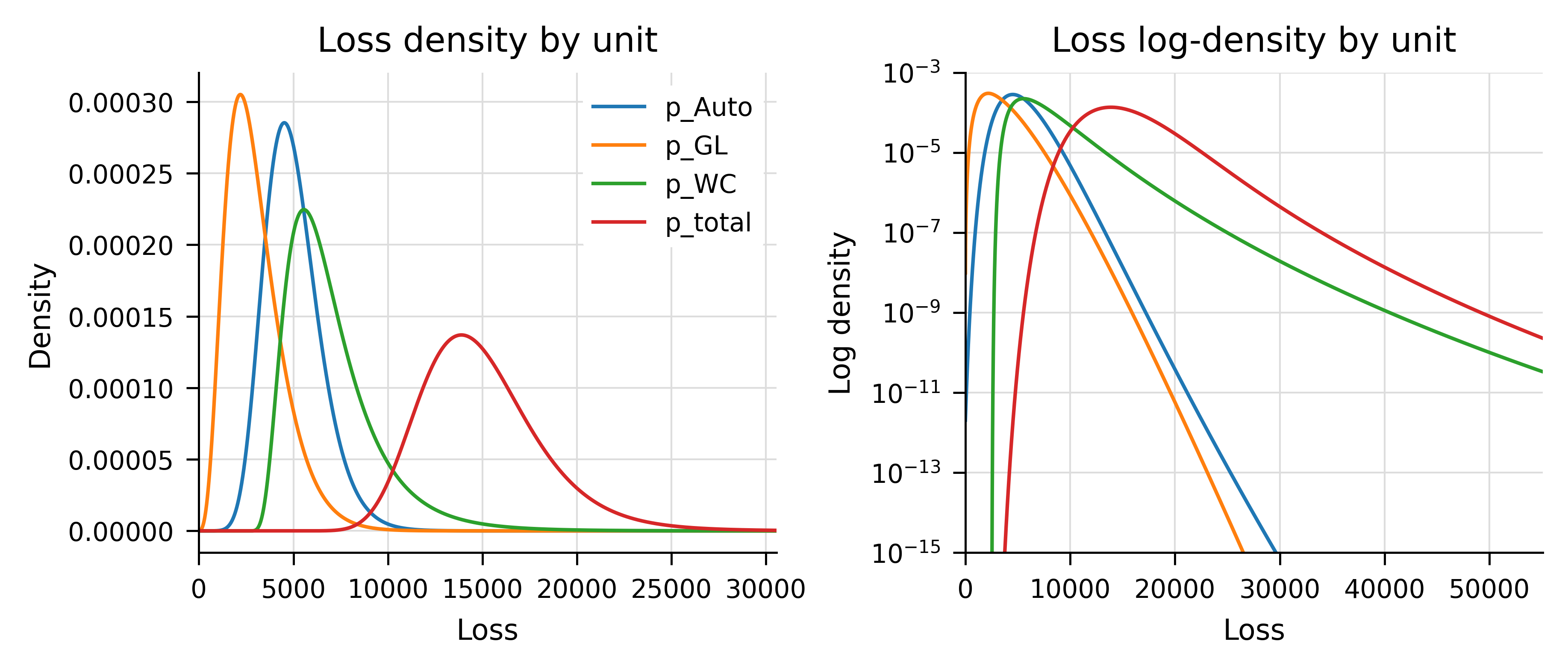
Table 9.11 shows the by-unit frequency and severity statistics and the total statistics assuming the units are independent. The deviation between the Fast Fourier Transform-generated compound distributions and the requested specifications are negligible. Figure 9.2 plots the unit and total densities on a nominal and log scale. The effect of WC driving the tail, via thicker severity and higher occurrence limit, is clear on the log plot.
Table 9.11: Unit frequency, severity and compound assumptions, and portfolio total, showing requested and model achieved and key statistics.
unit
X
E[X]
Est E[X]
CV(X)
Est CV(X)
Skew(X)
Est Skew(X)
Auto
Freq
100.0
0
0.224
0
0.402
0
Sev
49.982
49.982
1.973
1.973
10.678
10.678
Agg
5,000
5000.0
0.298
0.298
0.699
0.699
GL
Freq
41.008
0
0.338
0
0.604
0
Sev
73.156
73.156
2.377
2.378
7.385
7.385
Agg
3,000
3000.0
0.502
0.502
1.024
1.024
WC
Freq
1401.1
0
0.251
0
0.500
0
Sev
4.996
4.945
9.103
9.198
147.9
147.9
Agg
7,000
7000.0
0.350
0.350
1.776
1.775
total
Freq
1542.1
0
0.229
0
0.496
0
Sev
9.727
9.681
6.123
0
68.886
0
Agg
15,000
15000.0
0.216
0.216
0.939
0.938
Figure 9.2: By-unit loss densities (left) and logdensities (right).
Next, we sample from the unit distributions and shuffle using Iman-Conover to achieve the desired correlation shown in Table 9.12. This matrix comes from a separate analysis. The revised statistics (note higher total CV), quantiles, and achieved correlation are shown in Table 9.13 and Table 9.14.
Table 9.12: Desired correlation matrix, as input to Iman-Conover.
index
Auto
GL
WC
Auto
1
0.5
0.4
GL
0.5
1
0.1
WC
0.4
0.1
1
Table 9.13: Key statistics from sample with Iman-Conover induced correlation.
index
Auto
GL
WC
Total
count
1,000
1,000
1,000
1,000
mean
5010.4
2991.9
6996.2
14998.6
std
1469.6
1488.6
2603.5
4065.6
min
1,722
469
3,293
7,156
25%
3977.8
1933.8
5267.2
12098.8
50%
4897.5
2742.5
6,387
14412.5
75%
5896.8
3781.2
8043.2
17272.5
max
11,136
11,249
31,008
42,501
CV
0.293
0.498
0.372
0.271
Table 9.14: Achived between-unit correlation.
index
Auto
GL
WC
Total
Auto
1
0.491
0.349
0.765
GL
0.483
1
0.072
0.590
WC
0.391
0.093
1
0.793
total
0.788
0.591
0.758
1
Table 9.15 shows the output of using the correlated sample to build a Portfolio object. This uses the samples directly, proxying the aggregate loss as a compound with degenerate frequency distribution identically equal to one and severity equal to the desired distribution. Hence the frequency rows show expectation one with zero CV.
Table 9.15: Portfolio statistics reflecting the correlation achieved by the Iman-Conover sample.
unit
X
E[X]
Est E[X]
CV(X)
Est CV(X)
Skew(X)
Est Skew(X)
Auto
Freq
1
0
Sev
5010.4
5010.4
0.293
0.293
0.636
0.636
Agg
5010.4
5010.4
0.293
0.293
0.636
0.636
GL
Freq
1
0
Sev
2991.9
2991.9
0.497
0.497
1.222
1.222
Agg
2991.9
2991.9
0.497
0.497
1.222
1.222
WC
Freq
1
0
Sev
6996.2
6996.2
0.372
0.372
2.202
2.202
Agg
6996.2
6996.2
0.372
0.372
2.202
2.202
total
Freq
3
0
Sev
4999.5
4999.5
0.505
1.487
Agg
14998.6
14998.6
0.223
0.223
1.206
1.206
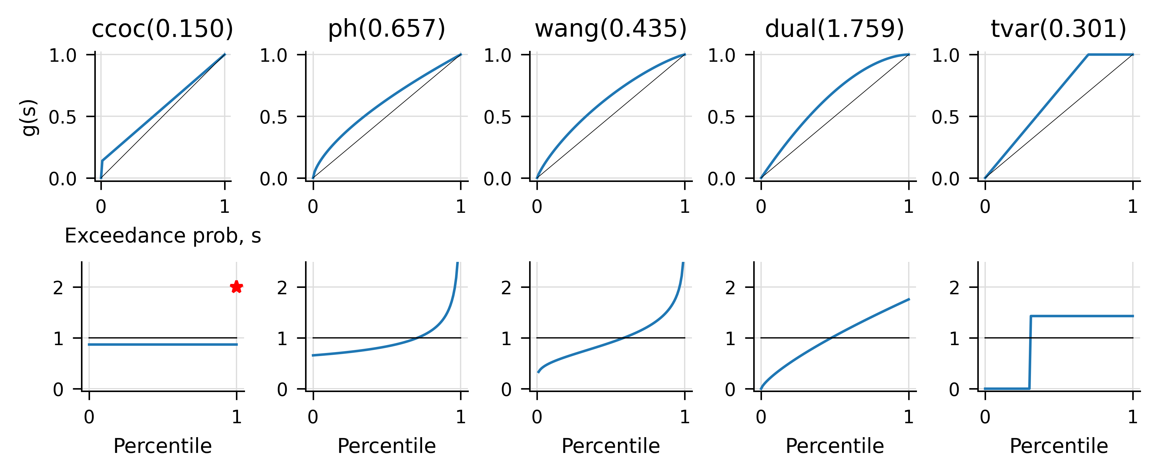
Table 9.16 shows the parameters for distortions calibrated to achieve an overall 15% return at a 99.5% capital standard. Figure 9.3 plots the distortions and probability adjustment functions, compare this with Figure 9.1. These distortions are slightly more risk averse (higher parameters except PH, driving higher indicated prices).
Table 9.16: Distortion parameters for to target total return at the regulatory capital standard.
method
P
param
error
ccoc
16777.2
0.150
0
ph
16777.2
0.657
0
wang
16777.2
0.435
0.000
dual
16777.2
1.759
-0.000
tvar
16777.2
0.301
0.000
Figure 9.3: Distortion functions and distortion probability adjustment functions.
Table 9.17 compares the indicated pricing by unit and distortion. It is computed using exactly the same method described for the simple discrete example. The calculations are easy enough that they can be performed in a spreadsheet, but that is not recommended unless you are very patient. Table 9.18 shows just the implied loss ratios. The total loss ratios are all the same because the distortions are all calibrated to the same overall total premium. Since WC has the heaviest tail, it gets the lowest target loss ratio under CCoC, which is the most tail-risk averse. In fact, CCoC is so tail-risk averse that GL (which offers some diversification because of the correlation structure) gets a target over 100%. This is typical CCoC behavior—cat is really expensive; everything else is cheaper. The reason is clear when you remember CCoC pricing is just a weighted average of the mean and the max. The other distortions are more reasonable. TVaR and dual are quite similar and focus more on volatility risk. Since all three lines are similarly volatile, it is no surprise their target loss ratios are also similar under this view.
This analysis—and indeed the whole monograph—has ignored several important elements: expenses, taxes, and the time value of money. Expenses are relatively easy to incorporate: acquisition expenses are typically amortized over the policy term, administration expenses span the policy term and claim payout period, and claim expenses can be bundled with losses. Taxes, however, are a Byzantine labyrinth requiring careful modeling at the level of legal entity and country. Their treatment is up to each insurer, and it’s hard to offer even vague general guidance. Finally, time value of money brings real conceptual and computational difficulty (as opposed to the man-made complexity of taxes). It is the quantum gravity of insurance pricing. For some early thoughts, see the forthcoming monograph Pricing Multi-Period Insurance Risk by your intrepid second author.
Table 9.17: Pricing by distortion.
(a) CCoC
statistic
Auto
GL
WC
Total
L
5007.2
2990.0
6984.5
14981.7
a
5780.1
3351.0
19615.9
28747.0
Q
783.1
380.0
10806.7
11969.8
P
4997.0
2971.0
8809.1
16777.2
M
-10.134
-19.019
1824.6
1795.5
COC
-0.013
-0.050
0.169
0.150
(b) PH
statistic
Auto
GL
WC
Total
L
5007.2
2990.0
6984.5
14981.7
a
8632.6
5552.1
14562.3
28747.0
Q
3189.4
2214.4
6566.0
11969.8
P
5443.2
3337.7
7996.3
16777.2
M
436.0
347.7
1011.8
1795.5
COC
0.137
0.157
0.154
0.150
(c) Wang
statistic
Auto
GL
WC
Total
L
5007.2
2990.0
6984.5
14981.7
a
8952.3
5686.4
14108.3
28747.0
Q
3451.3
2308.1
6210.4
11969.8
P
5501.0
3378.3
7897.9
16777.2
M
493.8
388.3
913.4
1795.5
COC
0.143
0.168
0.147
0.150
(d) Dual
statistic
Auto
GL
WC
Total
L
5007.2
2990.0
6984.5
14981.7
a
9081.1
5759.9
13906.0
28747.0
Q
3536.2
2354.4
6079.2
11969.8
P
5544.9
3405.5
7826.8
16777.2
M
537.7
415.5
842.3
1795.5
COC
0.152
0.176
0.139
0.150
(e) TVaR
statistic
Auto
GL
WC
Total
L
5007.2
2990.0
6984.5
14981.7
a
9129.4
5782.5
13835.1
28747.0
Q
3546.4
2355.2
6068.2
11969.8
P
5583.0
3427.3
7766.9
16777.2
M
575.8
437.3
782.4
1795.5
COC
0.162
0.186
0.129
0.150
Table 9.18: Implied loss ratio by unit by pricing by distortion (extract from previous tables).
Method
Auto
GL
WC
Total
Dist ccoc
100.2%
100.6%
79.3%
0.893
Dist ph
92.0%
89.6%
87.3%
0.893
Dist wang
91.0%
88.5%
88.4%
0.893
Dist dual
90.3%
87.8%
89.2%
0.893
Dist tvar
89.7%
87.2%
89.9%
0.893
Mildenhall, Stephen J. 2024. “Aggregate: fast, accurate, and flexible approximation of compound probability distributions.”Annals of Actuarial Science, 1–40. https://doi.org/10.1017/S1748499524000216.
Mildenhall, Stephen J, and John A Major. 2022. Pricing Insurance Risk: Theory and Practice. John Wiley & Sons, Inc.
Source Code
---format: pdf: default html: defaultjupyter: jupytext: text_representation: extension: .qmd format_name: quarto format_version: '1.0' jupytext_version: 1.16.4 kernelspec: display_name: Python 3 (ipykernel) language: python name: python3---```{python}#| echo: false#| label: spacerpass```# Calculations with `Aggregate` {#sec-Calcs-with-Aggregate}*Example calculations using Python and R.*This chapter reproduces many of the exhibits from the main text using Python and the `aggregate` package. It also describes how to extend to more realistic examples. Throughout, we have included only terse subsets of code so the reader can focus on the results and the output. Instructions for obtaining the full code are provided below.## `Aggregate` and Python`aggregate` is a Python package that can be used to build approximations to compound (aggregate) probability distributions quickly and accurately, and to solve insurance, risk management, and actuarial problems using realistic models that reflect underlying frequency and severity. It delivers the speed and accuracy of parametric distributions to situations that usually require simulation, making it as easy to work with an aggregate (compound) probability distribution as the lognormal. `aggregate` includes an expressive language called DecL to describe aggregate distributions.The `aggregate` package is available on [PyPi](https://pypi.org/project/aggregate/), the source code is on GitHub at <https://github.com/mynl/aggregate>, and there is extensive [documentation](https://aggregate.readthedocs.io/en/latest/). The `Aggregate` class and DecL lanaguage are described in @Mildenhall2024. There is also an extensive series of videos introducing various capabilities available on [YouTube](https://www.youtube.com/playlist?list=PLQQxycbewjqMDmw0hfZdB6Rzm60Qcq3Ao).## `Aggregate` and RPython packages can be used in R via the reticulate library. Python and R code can also be mixed in RMarkdown (now Quarto) files. This [short video](https://www.youtube.com/watch?v=jA9rVMHVqI0) explains how to use `aggregate` from R.## Reproducing the code examples {#sec-setup-code}To reproduce the Python code examples, you must set up your environment and then install `aggregate` using``` pythonpip install aggregate```The formatting of the examples relies on `greater_tables`, which can be installed in the same way. The installation process will also install several standard packages, such as `numpy` and `pandas`, that it depends on. If you get an error message about other missing packages, you can install them with `pip`. All the code in the monograph runs on `aggregate` version 0.24.0 and should run on any later version. If you have an older version installed, you can updated it with `pip install -U aggregate`.Once `aggregate` is installed, start by importing basic libraries. The next code block shows the relevant `aggregate` function. The class `GT` from `greater_tables` is used to format DataFrames consistently.``` pythonfrom aggregate import ( Portfolio, # creates multi-unit portfolios make_ceder_netter, # models reinsurance Distortion # creates a Distortion function)from greater_tables import GT # consistent table format``````{python}#| echo: false#| label: lstx-setup-code%run prefob.py# column ordering to match remainder of Monographjam_order = ['L', 'a', 'Q', 'P', 'M', 'COC']```\medskip**Online resources.** Complete code samples can be extracted from the online version of the monograph, available at <https://cmm.mynl.com/>. Each code block has a small copy icon in the upper right-hand corner. The code blocks on each page can all be shown or hidden using the `</>Code` control at the top of the page. To download the original qmd file, use the View Source option under the same control. Alternatively, the entire Quarto (previously RMarkdown) source can be downloaded from GitHub at https://github.com/mynl/CapitalModeling (CAS TO INSERT OWN LINK).## Reproducing the discrete example {#sec-sde}### Input data and setupThe InsCo example running through this monograph is based on the 10 events shown in @tbl-10-sims, which reproduces @tbl-dupe-x, and adds the mean and CV. For reference, here is the code to create the underlying dataframe.```{python}#| echo: true#| label: lstx-loss-sampleloss_sample = pd.DataFrame( {'A': [ 5, 7, 15, 15, 13, 5, 15, 26, 17, 16],'B': [20, 33, 13, 7, 20, 27, 16, 19, 8, 20],'C': [11, 0, 0, 0, 7, 8, 9, 10, 40, 64], })loss_sample['total'] = loss_sample.sum(axis=1)loss_sample['p_total'] =1/10print(loss_sample)``````{python}#| echo: false#| label: tbl-10-sims#| tbl-cap: The 10 equally likely simulations underlying the basic examples.loss_sample = pd.DataFrame( {'A': [ 5, 7, 15, 15, 13, 5, 15, 26, 17, 16],'B': [20, 33, 13, 7, 20, 27, 16, 19, 8, 20],'C': [11, 0, 0, 0, 7, 8, 9, 10, 40, 64],'p_total': 1/10 })loss_sample['total'] = loss_sample.iloc[:, :3].sum(1)# add mean and CVwgs = loss_sample.copy()wgs_ = wgs.copy().drop(columns='p_total')wgs_['total'] = wgs.drop(columns='p_total').sum(1)wgs2 = wgs_.copy()wgs2.loc['EX', :] = wgs_.mean(0)wgs2.loc['EX2', :] = (wgs_**2).mean(0)wgs2.loc['Var', :] = wgs2.loc['EX2', :] - wgs2.loc['EX', :]**2wgs2.loc['CV', :] = wgs2.loc['Var', :]**.5/ wgs2.loc['EX', :]wgs2 = wgs2.drop(index = ['EX2', 'Var'])fGT(wgs2)```Now we create an `aggregate``Portfolio` class instance based on the `loss_sample` simulation output. The next block shows how to do this, using the `Portfolio.create_from_sample` method. `TMA1` is a label, and `loss_sample` is the dataframe created previously. The other arguments specify working with unit-sized buckets `bs=1` appropriate for our integer losses and to use $256=2^8$ buckets, `log2=8`.```{python}#| echo: true#| label: lstx-create-portwport = Portfolio.create_from_sample('TMA1', loss_sample, bs=1, log2=8)```The next line of code displays @tbl-wport, which shows summary output from the object `wport` by accessing its `describe` attribute. The summary includes the mean, CV, and skewness. The model and estimated (`Est`) columns are identical because we specified the distribution directly; no simulation or Fast Fourier Transform-based numerical methods are employed.```{python}#| echo: true#| label: tbl-wport#| tbl-cap: Summary statistics for the base example.fGT(wport.describe.drop(columns=['Err E[X]', 'Err CV(X)']))```Next, we need to calibrate distortion functions to achieve the desired pricing. The example uses full capitalization throughout (assets equal the maximum loss), which is equivalent to a 100% percentile level (see @tbl-quantiles) and assumes the cost of capital is 15%. The code runs the calibration by calling `wport.calibrate_distortions` with arguments for the capital percentile level `Ps` and cost of capital `COCs`. The arguments are passed as lists because the routine can be used to solve for several percentile levels and costs simultaneously. @tbl-9-1 shows the resulting parameters, which match those in @tbl-the5dists.```{python}#| echo: true#| label: lstx-9-1# calibrate to 15% return at p=100% capital standardwport.calibrate_distortions(Ps=[1], COCs=[.15]);``````{python}#| echo: false#| label: tbl-9-1#| tbl-cap: "Distortion functions calibrated to 15% return on full capital."fGT(wport.distortion_df[['P', 'param', 'error']].droplevel([0, 1], 0))```@fig-distortion-functions shows the resulting distortion $g$ functions (top) and the probability adjustment $Z=q/p$ (bottom). The red star indicates a probability mass at $p=1$.```{python}#| echo: false#| label: fig-distortion-functions#| fig-cap: Distortion functions (top row) and distortion probability adjustment functions (bottom row).fig, axs = plt.subplots(2, 5, figsize=(5*1.25, 2*1.25), constrained_layout=True, sharey=False, sharex=False)axi0 =iter(axs[0])axi1 =iter(axs[1])xs = np.linspace(0, 1, 101)for (k, v), ax1, ax inzip(wport.dists.items(), axi0, axi1):if k =='ccoc': ax.plot([0,1], [1/1.15]*2) ax.plot(1, 2, 'r*')else: ax.plot(xs, v.g_prime(xs[::-1])) ax.plot([0, 1], [1,1], lw=.5, c='k') ax.set(ylim=[-0.05, 2.5])if ax is axs[1][0]: ax.set(ylabel='Z', xlabel='Percentile') ax1.plot(xs, v.g(xs)) ax1.plot([0, 1], [0, 1], 'k', lw=.25) k =f'{k}({v.shape:.3f})' ax1.set(title=k, ylim=[-0.025, 1.025])if ax1 is axs[0][0]: ax1.set(xlabel='Exceedance prob, s', ylabel='g(s)', aspect='equal')```For technical reasons (discussed in @sec-Complications as well as chapter 14.1.5 in @PIR, see especially Figure 14.2), we must summarize the 10 events by distinct totals. Routine code produces @tbl-5-1, reproducing @tbl-abc-x. <!--# In Table 9.4, the data in the row for index 3 go to the thousandths, while the other rows at most go to tenths. Suggest revising the data in row Index 3 so that it is similar to that of other rows. -->```{python}#| echo: false#| label: tbl-5-1#| tbl-cap: Assumptions for portfolio, summarized by distinct totals.bit = loss_sample.copy()bit['Total'] = bit[['A','B','C']].sum(axis=1)bit = bit.sort_values('Total')bit2 = bit.groupby('Total').apply(# [[]].values -> column vector to broadcast correctlylambda grp: (grp[['A', 'B', 'C']] * grp[['p_total']].values).sum() / grp['p_total'].sum() )bit2['p'] = bit.groupby('Total').apply(lambda grp: grp[['p_total']].sum())bit2 = bit2.reset_index(drop=True)bit2.loc['EX'] = bit.mean(0)bit2.loc['EX', 'p'] =1bit2.loc['Plan'] = [13.9, 18.7, 19.6, 1]bit2['Total'] = bit2[['A','B','C']].sum(1)fGT(bit2)```The examples describe a VaR- or TVaR-based capital standard (see @tbl-CA-loss-levels), but for this example it works out to the the same as a fully capitalized 100% standard, as shown by the values in @tbl-quantiles. The `wport` methods `q` and `tvar` compute quantiles and TVaRs for each unit and the total.```{python}#| echo: false#| label: tbl-quantiles#| tbl-cap: Quantiles (VaR) and TVaR at different probability levels.ps = [.8, .85, .9, 1]fGT(pd.DataFrame({'p': ps, 'Quantile': wport.q(ps),'TVaR': wport.tvar(ps)}).set_index('p'))```### Premiums by distortion@tbl-isa-alloc shows premium assuming a CCoC distortion with a 15% return applied using a 100% capital standard. The premium `P` row shows what @PIR calls the linear NA premium. @tbl-ccoc-na reproduces this exhibit, confirming an equal 15% returns across all allocated capital. The code illustrates the power of `aggregate`. The first line creates a CCoC distortion using the `Distortion` class; note the argument is risk discount $\delta$. The second line uses the `price` method to compute the linear allocation, which it returns in a structure with various diagnostic information, including @tbl-ccoc-na. <!--# In Table 9.6, I would capitalize "Total," so it matches the style of other tables. -->```{python}#| echo: true#| label: lstx-ccoc-na-0ccoc = Distortion.ccoc(.15/1.15)pricing_info = wport.price(1, ccoc, allocation='linear')``````{python}#| echo: false#| label: tbl-ccoc-na#| tbl-cap: Industry standard approach pricing using the CCoC distortion.# best to drop the multi-index columnsfGT(pricing_info.df[jam_order].T.droplevel(0, 1), aligners={c: 'r'for c in jam_order})```@tbl-x-collapsed, @tbl-ccoc-1 and @tbl-ccoc-qx compute $\rho(X)$ for $\rho$ the CCoC SRM, using the $\rho(X)=\int g(S(x))\,dx$ (second table) and $\rho(X)=\int xg'(S(x))f(x)\,dx$ (third) representations. The numbers needed for these calculations are shown in @tbl-gs-calcs, where $q=g'(S(x))f(x)$. These are extracted from the dataframe `wport.density_df,` which contains the probability mass, density, and survival functions for the portfolio, among other facts. The last row carries out the calculations and confirms the two methods give the same result, the total under $gS$ using the former representation and under $q$ using the latter representation.```{python}#| echo: false#| label: tbl-gs-calcs#| tbl-cap: "Industry standard approach pricing: raw ingredients and computed means."bit = wport.density_df.query('p_total > 0')[['p_total', 'F', 'S']]bit['gS'] = ccoc.g(bit.S)bit['q'] =-np.diff(bit.gS, prepend=1)bit['ΔX'] = np.diff(bit.index, append=100)bit.index.name ='loss'eq = (bit.index * bit.q).sum()gsdx = (bit.gS.iloc[:-1] * np.diff(bit.index)).sum() + bit.index[0]bit.loc['$\\rho(X)$'] =''bit.loc['$\\rho(X)$', 'q'] = eqbit.loc['$\\rho(X)$', 'gS'] = gsdxfGT(bit, aligners={c:'r'for c in bit.columns})```<!-- @tbl-Wang-alloc shows the results of using the Wang distortion in place of the CCoC. -->@tbl-all-distortion-pricing shows the results for the other standard distortions. The calculations match those of the Wang in @tbl-all-distortion-pricing-3. All of the calibrated distortions are carried in the dictionary `wport.dists`. These tables also include the NA of capital (a process we do not recommend, but that is described in @sec-Allocating-Capital). The `Q` row matches the calculation of allocated capital shown in @tbl-q-alloc. <!--# In Table 9.8, I also recommend capitalizing "Total" in the fourth column all all panels for consistency. -->```{python}#| echo: false#| label: tbl-all-distortion-pricing#| tbl-cap: Pricing by distortion by unit.#| layout-ncol: 1#| tbl-subcap: [CCoC, PH, Wang, Dual, TVaR]for k, g in wport.dists.items(): display(fGT( wport.price(1, g, allocation='lifted').df[jam_order].T.droplevel(0, 1)))```### Reinsurance analysis@sec-Applications analyzes a possible 35 xs 65 aggregate stop loss reinsurance contract. The setup to analyze this contract, using a separate `Portfolio` object, is shown next. The first two lines apply reinsurance; `[1, 35, 65]` specifies 100% of the 35 xs 65 layer, and `c` and `n` are functions mapping gross to ceded and net. The last line creates a new `Portfolio` object from the net and ceded aggregate losses.```{python}#| echo: true#| label: lstx-setup-reloss_sample_re = loss_sample.copy()c, n = make_ceder_netter([(1, 35, 65)])loss_sample_re['Net'] = n(loss_sample_re.total)loss_sample_re['Ceded'] = c(loss_sample_re.total)loss_sample_re = loss_sample_re[['Net', 'Ceded', 'p_total']]# build Portfolio object with Net, Ceded unitswport_re = Portfolio.create_from_sample('WGS3', loss_sample_re[['Net', 'Ceded', 'p_total']], bs=1, log2=8)```@tbl-re-object shows the standard summary statistics. <!--# In Table 9.9, for consistency, I would capitalize "total" in column 1. --> It should be compared to @tbl-events-with-RI. @tbl-all-distortioun-re-pricing shows the allocated pricing to the reinsurance and net across the five standard distortions, compare with the last row of @tbl-events-with-RI and discussion in @sec-Reinsurance-decision-making. <!--# In Table 9.10, recommend capitalizing "total" in the far right column of the header row. -->```{python}#| echo: false#| label: tbl-re-object#| tbl-cap: "Summary statistics created by the reinsurance Portfolio object."fGT(wport_re.describe.drop(columns=['Err E[X]', 'Err CV(X)']))``````{python}#| echo: false#| label: tbl-all-distortioun-re-pricing#| tbl-cap: Pricing by distortion for ceded, net, and total (gross).#| layout-ncol: 1#| tbl-subcap: [CCoC, PH, Wang, Dual, TVaR]for k, g in wport.dists.items(): display(fGT(wport_re.price(1, g, allocation='lifted').df[jam_order].T.droplevel(0, 1)))```\clearpage## A more realistic example {#sec-realistic}In this section, we create a series of exhibits analogous to those in @sec-sde for an example with more realistic assumptions. It is included to show how `aggregate` can be used to solve real-world problems, hopefully motivating you to explore it further. The analysis steps are:1. Create realistic by-unit frequency and severity distributions using Fast Fourier Transforms with independent units.2. Sample the unit distributions with correlation induced by Iman-Conover, @sec-iman-conover.3. Build a `Portfolio` from the correlated sample.4. Calibrate distortions and compute unit pricing for each distortion.5. Apply by-unit, per-occurrence reinsurance and examine pricing impact.The `aggregate` DecL programming language makes it easy to specify frequency-severity compound distributions. In the code chunk below, the four lines inside the `build` statement are the DecL program. The triple quotes are Python shorthand for entering a multiline string. The first program line, beginning `agg Auto`, creates a distribution with an expected loss of 5000 (think: losses in 000s), severity from the 5000 xs 0 layer of a lognormal variable with a mean of 50 and a CV of 2, and gamma mixed-Poisson frequency with a mixing parameter (CV) of 0.2. The other two lines are analogous. The `build` statement runs the DecL program and creates a `Portfolio` object with relevant compound distributions by unit. It also sums the unit distributions as though they were independent---we will introduce some correlation later.```{python}#| echo: true#| label: lstx-univariates-0from aggregate import buildport = build("""port Units agg Auto 5000 loss 5000 xs 0 sev lognorm 50 cv 2 mixed gamma 0.2 agg GL 3000 loss 2500 xs 0 sev lognorm 75 cv 3 mixed gamma 0.3 agg WC 7000 loss 25000 xs 0 sev lognorm 5 cv 10 mixed gamma 0.25""")```@tbl-univariates-1 shows the by-unit frequency and severity statistics and the total statistics assuming the units are independent. The deviation between the Fast Fourier Transform-generated compound distributions and the requested specifications are negligible. @fig-univariates plots the unit and total densities on a nominal and log scale. The effect of WC driving the tail, via thicker severity and higher occurrence limit, is clear on the log plot. <!--# In Table 9.11, recommend capitalizing "Total." -->```{python}#| echo: false#| label: tbl-univariates-1#| tbl-cap: "Unit frequency, severity and compound assumptions, and portfolio total, showing requested and model achieved and key statistics."fGT(port.describe.drop(columns=['Err E[X]', 'Err CV(X)']).fillna(0))``````{python}#| echo: false#| label: fig-univariates#| fig-cap: By-unit loss densities (left) and logdensities (right).fig, axs = plt.subplots(1, 2, figsize=(6, 2.5), constrained_layout=True)ax0, ax1 = axs.flatbit = port.density_df[[f'p_{i}'for i in port.unit_names_ex]]bit.plot(ax=ax0)ax0.set(title='Loss density by unit', xlim=[0, port.q(0.999)], xlabel='Loss', ylabel='Density')bit = port.density_df[[f'p_{i}'for i in port.unit_names_ex]]bit.plot(ax=ax1)ax1.legend().set(visible=False)ax1.set(title='Loss log-density by unit', xlim=[0, port.q(0.999999)], xlabel='Loss', yscale='log', ylabel='Log density', ylim=[1e-15, 1e-3]);```Next, we sample from the unit distributions and shuffle using Iman-Conover to achieve the desired correlation shown in @tbl-correl. This matrix comes from a separate analysis. The revised statistics (note higher total CV), quantiles, and achieved correlation are shown in @tbl-stats-sample and @tbl-correl-sample. <!--# In Table 9.14, recommend capitalizing "Total." -->```{python}#| echo: false#| label: tbl-correl#| tbl-cap: "Desired correlation matrix, as input to Iman-Conover."desired_corr = np.array([[1., .5, .4], [.5, 1., .1], [.4, .1, 1.]])fGT(pd.DataFrame(desired_corr, index=port.unit_names, columns=port.unit_names))``````{python}#| echo: false#| label: tbl-stats-sample#| tbl-cap: 'Key statistics from sample with Iman-Conover induced correlation.'sample = port.sample(1000, desired_correlation=desired_corr)sample['total'] = sample.sum(1)st = sample.describe()st.loc['CV'] = st.loc['std'] / st.loc['mean']display(fGT(st))``````{python}#| echo: false#| label: tbl-correl-sample#| tbl-cap: 'Achived between-unit correlation.'lin = sample.corr()rk = sample.corr('spearman')mask = np.tril(np.ones(rk.shape), k=-1)==1fGT(lin.where(~mask, other=0) + rk.where(mask, other=0))```@tbl-univariates-corr shows the output of using the correlated sample to build a `Portfolio` object. <!--# In Table 9.15, recommend capitalizing "Total." -->This uses the samples directly, proxying the aggregate loss as a compound with degenerate frequency distribution identically equal to one and severity equal to the desired distribution. Hence the frequency rows show expectation one with zero CV.```{python}#| echo: false#| label: tbl-univariates-corr#| tbl-cap: "Portfolio statistics reflecting the correlation achieved by the Iman-Conover sample."port_corr = Portfolio.create_from_sample('UnitsCorr', sample, bs=port.bs, log2=port.log2)fGT(port_corr.describe.drop(columns=['Err E[X]', 'Err CV(X)']))```@tbl-param-d shows the parameters for distortions calibrated to achieve an overall 15% return at a 99.5% capital standard. @fig-distortion-functions-sample plots the distortions and probability adjustment functions, compare this with @fig-distortion-functions. These distortions are slightly more risk averse (higher parameters except PH, driving higher indicated prices).```{python}#| echo: false#| label: tbl-param-d#| tbl-cap: "Distortion parameters for to target total return at the regulatory capital standard."reg_p =0.995# regulatory capital standardwacc =0.15# computed total weighted average cost of capitalport_corr.calibrate_distortions(Ps=[reg_p], COCs=[wacc])fGT(port_corr.distortion_df[['P', 'param', 'error']].droplevel([0, 1], 0))``````{python}#| echo: false#| label: fig-distortion-functions-sample#| fig-cap: Distortion functions and distortion probability adjustment functions.fig, axs = plt.subplots(2, 5, figsize=(5*1.25, 2*1.25), constrained_layout=True, sharey=False, sharex=False)axi0 =iter(axs[0])axi1 =iter(axs[1])xs = np.linspace(0, 1, 101)for (k, v), ax1, ax inzip(port_corr.dists.items(), axi0, axi1):if k =='ccoc': ax.plot([0,1], [1/(1+ wacc)]*2) ax.plot(1, 2, 'r*')else: ax.plot(xs, v.g_prime(xs[::-1])) ax.plot([0, 1], [1,1], lw=.5, c='k') ax.set(ylim=[-0.05, 2.5], xlabel='Percentile')if ax is axs[0]: ax.set(ylabel='Weight adjustment') ax1.plot(xs, v.g(xs)) ax1.plot([0, 1], [0, 1], 'k', lw=.25) k =f'{k}({v.shape:.3f})' ax1.set(title=k, ylim=[-0.025, 1.025])if ax1 is axs[0][0]: ax1.set(xlabel='Exceedance prob, s', ylabel='g(s)', aspect='equal')```@tbl-all-distortion-realistic-pricing compares the indicated pricing by unit and distortion. <!--# In Table 9.17, recommend capitalizing "Total" in header row. -->It is computed using exactly the same method described for the simple discrete example. The calculations are easy enough that they can be performed in a spreadsheet, but that is not recommended unless you are very patient. @tbl-loss-ratios shows just the implied loss ratios. The total loss ratios are all the same because the distortions are all calibrated to the same overall total premium. Since WC has the heaviest tail, it gets the lowest target loss ratio under CCoC, which is the most tail-risk averse. In fact, CCoC is so tail-risk averse that GL (which offers some diversification because of the correlation structure) gets a target over 100%. This is typical CCoC behavior---cat is really expensive; everything else is cheaper. The reason is clear when you remember CCoC pricing is just a weighted average of the mean and the max. The other distortions are more reasonable. TVaR and dual are quite similar and focus more on volatility risk. Since all three lines are similarly volatile, it is no surprise their target loss ratios are also similar under this view.This analysis---and indeed the whole monograph---has ignored several important elements: expenses, taxes, and the time value of money. Expenses are relatively easy to incorporate: acquisition expenses are typically amortized over the policy term, administration expenses span the policy term and claim payout period, and claim expenses can be bundled with losses. Taxes, however, are a Byzantine labyrinth requiring careful modeling at the level of legal entity and country. Their treatment is up to each insurer, and it's hard to offer even vague general guidance. Finally, time value of money brings real conceptual and computational difficulty (as opposed to the man-made complexity of taxes). It is the quantum gravity of insurance pricing. For some early thoughts, see the forthcoming monograph Pricing Multi-Period Insurance Risk by your intrepid second author. <!--# Is there a prepublication link or something we can place here? Or even an entry in the references? -->```{python}#| echo: false#| label: tbl-all-distortion-realistic-pricing#| tbl-cap: Pricing by distortion.#| layout-ncol: 1#| tbl-subcap: [CCoC, PH, Wang, Dual, TVaR]for k, g in port_corr.dists.items(): display(fGT( port_corr.price(reg_p, g, allocation='lifted').df[jam_order].T.droplevel(0, 1) ))``````{python}#| echo: false#| label: tbl-loss-ratios#| tbl-cap: "Implied loss ratio by unit by pricing by distortion (extract from previous tables)."ansd = port_corr.analyze_distortions(p=reg_p, efficient=True, add_comps=False)bit = ansd.comp_df.xs('LR', 0, 1)bit = bit.iloc[[0, 2, 4, 1, 3]]fGT(bit, ratio_cols=['Auto', 'GL', 'WC', 'total'])```