8 Advanced topics
8.1 Dealing with uncertainty
In this world, nothing is certain except death and taxes.
- Benjamin Franklin, letter to Jean-Baptiste Leroy
The purpose of simulation is to estimate certain quantities of interest or QoI. A QoI is typically a quantile or other function (e.g., mean, risk measure) of the sample outcomes that the simulation created. Since it is being estimated from a sample, it cannot be measured with perfect accuracy because of sampling error. The more simulated samples are created, the more accurate the estimate can be. However, there is another reason that the estimate will not be accurate.
Parameter uncertainty here is to be distinguished from process risk. For example, when you simulate the outcome from a random variable with a lognormal distribution with particular parameters, you are modeling process risk. When you aren’t sure what the parameter values should be, you are suffering from parameter uncertainty. The uncertainty around input parameters will propagate to uncertainty about the QoI. For example, it is well known that ignoring parameter uncertainty often systematically biases estimated quantiles downward. See Jewson et al. (2025) for an approach to adjust for this bias.
Parameter uncertainty arises from nonsampling error. There are many potential sources of this in a capital model. Data used to build the model could have erroneous entries, or it might not be of an appropriate vintage or refer to a population that is sufficiently relevant to the modeling task. In building the model, perhaps not all relevant factors have been taken into account. This is not an exhaustive list!
In addition, some parameters vary over time. A data snapshot taken to estimate parameters may be inappropriate to modeling the same phenomenon at a later date.
Parameter uncertainty will likely permeate your modeling efforts, especially if you are trying to make a model that can replicate historical experience. There are several ways to deal with uncertainty:
- Ignore it. Use a best estimate of parameter values and let it go at that. While this may be acceptable for early versions of the model, it is not recommended for the long term. At the very least you must disclose that there is some uncertainty as to the QoI values and what the business risks of that are. “The answer is \(A\), but there is some uncertainty.”
- Report it. Statistical analysis of data will usually give some indication of the range (e.g., variance) of parameter values consistent with a chosen model for the data. If you want to push your luck, that insight can be turned into a distributional model for the parameters. Rerun your model with carefully chosen exemplars or a sample from the putative distribution of those random parameters. Report the range or the resulting distribution of the QoI. “The answer is \(A \pm \epsilon\).”
- Absorb it. Classical (frequentist) statistics has prediction intervals to accommodate uncertainty in the parameters; Bayesian theory provides a formal framework for treating parameter uncertainty as another species of process risk. Essentially, this means treating the random parameter as mixing the distribution of QoI, creating what Bayesians call a predictive distribution; see Bolstad and Curran (2016) or Geisser (2017). This is explained in an actuarial context in Kreps (1997); however, Major (1999) finds reasons to doubt it is always the right approach. Prediction intervals are bigger than classically estimated intervals. The QoI is likely to be sensitive to the upper tail, which moves up. “The answer is \(A+\delta\).”
- Isolate it. Find a credible worst-case to offer as an example of what can go wrong. This is the approach covered in Hansen and Sargent (2008) and Major et al. (2015). Again, this is likely to increase a risk-sensitive QoI. “The answer is \(A\), but it could be as bad as \(A+\gamma\).”
For a general treatment, see Smith (2024).
8.2 The Iman-Conover method
Correlation is not causation, but you can cause some correlation.
The Iman-Conover method is an easy way to induce correlation between marginal distributions. Here is the idea. Given samples of \(n\) values from \(r\) known marginal distributions \(X_1,\dots,X_r\) and a desired \(r\times r\) (linear) correlation matrix \(\Sigma\) between them, reorder the \(i\)th sample to have the same rank order as the \(i\)th column of a reference distribution of size \(n\times r\) with linear correlation \(\Sigma\). The reordered output will then have the same rank correlation as the reference, and since linear correlation and rank correlation are typically close, it will have close to the desired correlation structure. What makes the Iman-Conover method work so effectively is the existence of easy algorithms to determine samples from reference distributions with prescribed correlation structures.
The Iman-Conover method is very powerful, quick, and easy to use. However, it is not magic, and it is constrained by mathematical reality. For given pairs of distributions there is often an upper bound on the linear correlation between them, so if you ask for very high correlation you may be disappointed. You should go back and ask yourself why you think the linear correlation is so high.
Iman-Conover is usually used to induce a desired linear correlation. There other measures, such as rank correlation and Kendall’s tau, that could be used (Mildenhall 2005) and the user should reflect on which is most appropriate to their application. If your target is rank correlation, Iman-Conover will give you an exact match.
The aggregate documentation provides a detailed description of the algorithm, including discussion of using different reference distributions (called scores) in place of the normal, and a comparison with the normal copula method.
8.2.1 Loss or loss ratio?
Are you modeling correlation of loss ratios or correlation of losses? It is a surprising empirical fact that the former is often greater than the latter, leading to the conclusion that correlation in underwriting results is driven by correlation in premium more than loss, see Mildenhall (2022). These findings highlight a stark property-casualty split. Property tends to be loss-volatility driven, with loss correlation caused (and explained) by geographic proximity. Casualty tends to be premium-volatility driven, with loss ratio correlation caused by (account) underwriting and the underwriting cycle.
8.2.2 Example 1: A simple example
This section presents a simple example applying Iman-Conover to realistic distributions, using the aggregate library. It shows how easy it is to use Iman-Conover in modern programming languages. Another example, with more the details, appears in the aggregate documentation. See Section 9.3 for instructions to set up your Python environment to replicate the code samples. The full source code to replicate the examples is available on the Monograph website.
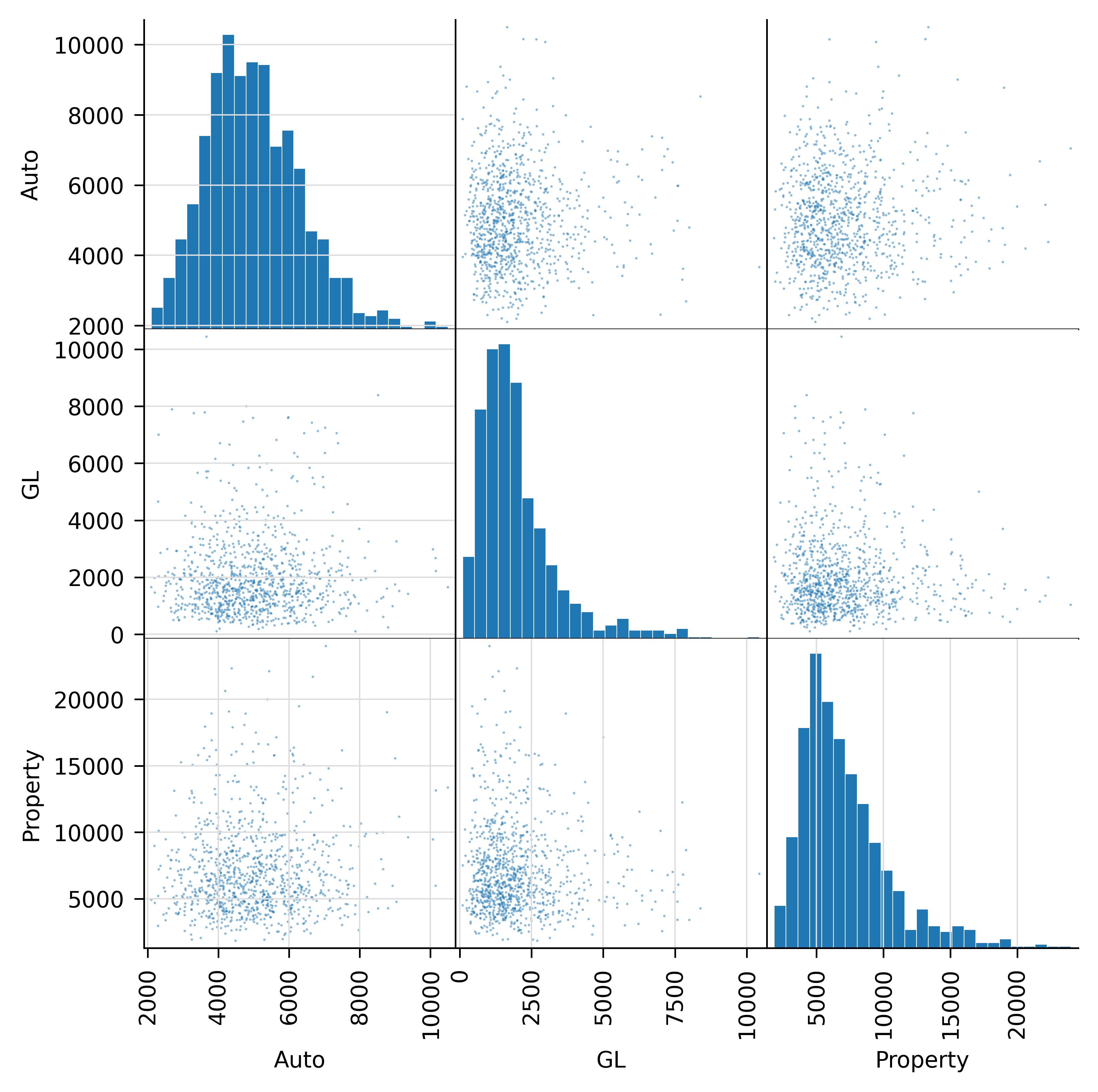
The example works with \(r=3\) different marginals: Auto, general liability (GL), and Property. Losses are simulated using frequency-severity aggregate distributions with a lognormal severity and per occurrence limits. Frequency is a gamma-mixed Poisson (negative binomial) with varying CVs. See Mildenhall (2023) for a description of the aggregate DecL language, used to specify these portfolios.
port ICExample
    agg Auto      5000 loss  2000 xs 0 sev lognorm  30 cv 2 mixed gamma 0.2
    agg GL        2000 loss  5000 xs 0 sev lognorm  50 cv 5 mixed gamma 0.3
    agg Property  7000 loss 10000 xs 0 sev lognorm 100 cv 5 mixed gamma 0.1
This example uses only 1,000 simulations, but the software can easily handle 100,000 or more. The slowest part of the Iman-Conover algorithm is creating the scores. These are cached, so subsequent runs are very fast, even if the desired correlation matrix changes.
Table 8.1 shows summary statistics and the first few samples of the underlying multivariate distribution, and Figure 8.1 shows histograms of each marginal and scatterplots. By construction, the units are approximately independent.
| index | Auto | GL | Property |
|---|---|---|---|
| count | 1,000 | 1,000 | 1,000 |
| mean | 5008.5 | 1995.3 | 7099.2 |
| std | 1340.3 | 1385.9 | 3375.5 |
| min | 2,104 | 101 | 1,833 |
| 25% | 4046.8 | 1066.8 | 4764.8 |
| 50% | 4917.5 | 1,644 | 6,296 |
| 75% | 5852.8 | 2,430 | 8,571 |
| max | 10,493 | 10,442 | 24,005 |
| cv | 0.268 | 0.695 | 0.475 |
| index | Auto | GL | Property |
|---|---|---|---|
| 0 | 3,328 | 1,248 | 7,966 |
| 1 | 5,950 | 841 | 6,929 |
| 2 | 4,455 | 2,117 | 7,250 |
| 3 | 5,466 | 941 | 4,084 |
| 4 | 6,232 | 5,368 | 5,071 |
| 5 | 4,371 | 2,301 | 15,818 |
| 6 | 4,323 | 1,689 | 6,439 |
| 7 | 4,528 | 1,405 | 8,243 |
| 8 | 4,568 | 738 | 7,287 |
| 9 | 4,946 | 959 | 10,724 |
In addition to marginal distributions, Iman-Conover requires a target desired correlation matrix as input. This is produced by a separate analysis, and here we assume it is given by Table 8.2. Remember, a correlation matrix must be symmetric (easy to check) and positive definite (harder). Matrices computed from statistical analysis may fail to be positive definite if they are not computed from a multivariate sample. Iman-Conover fails if given a nonpositive definite matrix.
| index | Auto | GL | Property |
|---|---|---|---|
| Auto | 1 | -0.3 | 0 |
| GL | -0.3 | 1 | 0.8 |
| Property | 0 | 0.8 | 1 |
The Iman-Conover method is implemented in aggregate by the function iman_conover, so the transformation is simply
where desired is the desired correlation matrix. Table 8.3 shows the achieved linear and rank correlation, and the absolute and relative errors. Finally, Figure 8.2 provides a scatter plot of the shuffled inputs, making the correlation evident. It is possible to obtain a correlated sample from a Portfolio object by passing in a correlation matrix: the code below extracts a sample and automatically applies Iman-Conover.
| index | Auto | GL | Property |
|---|---|---|---|
| Auto | 1 | -0.265 | 0.002 |
| GL | -0.265 | 1 | 0.774 |
| Property | 0.002 | 0.774 | 1 |
| index | Auto | GL | Property |
|---|---|---|---|
| Auto | 1 | -0.289 | 0.000 |
| GL | -0.289 | 1 | 0.790 |
| Property | 0.000 | 0.790 | 1 |
| index | Auto | GL | Property |
|---|---|---|---|
| Auto | 0 | 0.035 | 0.002 |
| GL | 0.035 | 0 | 0.026 |
| Property | 0.002 | 0.026 | 0 |
| index | Auto | GL | Property |
|---|---|---|---|
| Auto | 0 | -0.116 | inf |
| GL | -0.116 | 0 | -0.032 |
| Property | inf | -0.032 | 0 |

8.2.3 Different reference distributions
The Iman-Conover algorithm relies on a sample from a multivariate reference distribution called scores. A straightforward method to compute a reference is to use the Choleski decomposition method applied to certain independent scores (samples with mean zero and standard deviation one). The standard algorithm uses standard normal scores. However, nothing prevents the use of other distributions for the scores, provided they are suitably normalized to have mean zero and standard deviation one. Several other families of multivariate distributions could be used, such as elliptically contoured distributions (which include the normal and \(t\) as a special cases) and the multivariate Laplace distribution. These are all easy to simulate.
The aggregate implementation provides \(t\)-distribution scores. It includes an argument dof. By default dof=0 resulting in a normal reference. A dof>0 is interpreted as degrees of freedom, and the reference becomes a \(t\)-distribution. Figure 8.3 reruns Section 8.2.2 using a \(t\) reference with 2 degrees of freedom, a very extreme choice. It results in more tail correlation, evident in the pinched scatterplots. Be warned, however, that this modeling flexibility definitely falls into the “just because you can, doesn’t mean you should” category!

8.2.4 Copulas as reference distributions
The reader may be wondering about using a copula as a reference score. Alas, most copulas are only bivariate. Multivariate copulas, aside from those related to elliptical or Laplace distributions already mentioned, are Archimedian, which means they have a single parameter and cannot be calibrated to a desired correlation matrix.
See the aggregate documentation and Mildenhall (2005) for more details.
8.2.5 Iman-Conover compared with the normal copula method
The normal copula method is described in Wang (1998). Given a set of risks \((X_1,\dots,X_k)\) with marginal cumulative distribution functions \(F_i\) and Kendall’s tau \(\tau_{ij}=\tau(X_i,X_j)\) or rank correlation coefficients \(r(X_i,X_j)\), it works as follows. Assume that \((Z_1,\dots,Z_k)\) have a multivariate normal joint probability density function given by \[ f(z_1,\dots,z_k)=\frac{1}{\sqrt{(2\pi)^k|\Sigma|}}\exp(-\mathsf{z}'\Sigma^{-1}\mathsf{z}/2), \] \(\mathsf{z}=(z_1,\dots,z_k)\), with correlation coefficients \(\Sigma_{ij}=\rho_{ij}=\rho(Z_i,Z_j)\). Let \(H(z_1,\dots,z_k)\) be their joint cumulative distribution function. Then \[ C(u_1,\dots,u_k)=H(\Phi^{-1}(u_1),\dots,\Phi^{-1}(u_k)) \] defines a multivariate uniform cumulative distribution function called the normal copula. Using \(H\), the set of variables \[ X_1=F_1^{-1}(\Phi(Z_1)),\dots,X_k=F_1^{-1}(\Phi(Z_k)) \tag{8.1}\] have a joint cumulative function \[ F_{X_1,\dots,X_k}(x_1,\dots,x_k)=H(\Phi^{-1}(F_x(u_1)),\dots, \Phi^{-1}(F_k(u_k)) \] with marginal cumulative distribution functions \(F_1,\dots,F_k\). The multivariate variables \((X_1,\dots,X_k)\) have Kendall’s tau \[ \tau(X_i,X_j)=\tau(Z_i,Z_j)=\frac{2}{\pi}\arcsin(\rho_{ij}) \] and Spearman’s rank correlation coefficients \[ \text{rkCorr}(X_i,X_j)=\text{rkCorr}(Z_i,Z_j)=\frac{6}{\pi}\arcsin(\rho_{ij}/2) \] so \(\rho\) can be adjusted to achieve the desired correlation.
In the normal copula method, we simulate from \(H\) and then invert using Equation 8.1. In the Iman-Conover method with normal scores we produce a sample from \(H\) such that \(\Phi(z_i)\) are equally spaced between zero and one and then, rather than invert the distribution functions, we make the \(j\)th order statistic from the input sample correspond to \(\Phi(z)=j/(n+1)\) where the input has \(n\) observations. Because the \(j\)th order statistic of a sample of \(n\) observations from a distribution \(F\) approximates \(F^{-1}(j/(n+1))\), we see the normal copula and Iman-Conover methods are doing essentially the same thing.
While the normal copula method and the Iman-Conover method are confusingly similar, there are some important differences to bear in mind. Comparing and contrasting the two methods should help clarify how the two algorithms are different.
- Wang (1998) shows the normal copula method corresponds to the Iman-Conover method when the latter is computed using normal scores and the Choleski trick.
- The Iman-Conover method works on a given sample of marginal distributions. The normal copula method generates the sample by inverting the distribution function of each marginal as part of the simulation process.
- Through the use of scores, the Iman-Conover method relies on a sample of normal variables. The normal copula method could use a similar method, or it could sample randomly from the base normals. Conversely, a sample could be used in the Iman-Conover method.
- Only the Iman-Conover method has an adjustment to ensure that the reference multivariate distribution has exactly the required correlation structure.
- Iman-Conover method samples have rank correlation exactly equal to a sample from a reference distribution with the correct linear correlation. Normal copula samples have approximately correct linear and rank correlations.
- An Iman-Conover method sample must be taken in its entirety to be used correctly. The number of output points is fixed by the number of input points, and the sample is computed in its entirety in one step. Some Iman-Conover tools produce output, which is in a particular order. Thus, if you sample the \(n\)th observation from multiple simulations, or take the first \(n\) samples, you will not get a random sample from the desired distribution. However, if you select random rows from multiple simulations (or, equivalently, if you randomly permute the rows’ output prior to selecting the \(n\)th) then you will obtain the desired random sample. It is important to be aware of these issues before using canned software routines.
- The normal copula method produces simulations one at a time, and at each iteration the resulting sample is a sample from the required multivariate distribution. That is, output from the algorithm can be partitioned and used in pieces.
In summary, remember that these differences can have material, practical consequences, and it is important not to misuse Iman-Conover method samples.
8.2.6 Block Iman-Conover (BIC)
The Iman-Conover method can lead you into a state of sin: the sin of thinking you can reliably estimate a \(100 \times 100\) correlation matrix (or larger). You can’t; don’t try—it’s all noise. Look at the distribution of eigenvalues to see; start by computing the SVD and compare your distribution with that of a random matrix. However, you might be able to say something about the correlation of chunks of your book. Generally (going back to premium is riskier than loss), lines that are underwritten together have correlated loss ratios, and properties that are nearby have correlated losses. The Block Iman-Conover (BIC) method is a way to use this information without fabricating large correlation matrices.
8.2.6.1 Description of BIC
BIC is best explained through an example. You underwrite auto liability, GL, and property in four regions: North, East, South, and West. Based on reliable studies, you have a sense of the loss (ratio) correlation between each line overall (a \(3 \times 3\) matrix, with three parameters), and, separately, between the total regional results (a \(4 \times 4\) matrix, with six parameters). The BIC produces a multivariate sample across all 12 line and region units that incorporates what you know, but using just these nine parameters rather than requiring 66 parameters (for a \(12 \times 12\) matrix). Here’s how it works. Pick a number of simulations \(n\), then:
- Produce four \(n \times 3\) matrices with results by line for each region, \(R_1\), \(R_2\), \(R_3\), \(R_4\).
- Apply Iman-Conover to each \(R_i\) separately using your \(3\times 3\) between-line correlation matrix, to produce \(\tilde R_i\).
- Sum across simulations in each \(\tilde R_i\) to get total regional losses and assemble these into a \(n\times 4\) matrix \(T\).
- Apply Iman-Conover to \(T\) using your \(4\times 4\) between-region correlation matrix, and capture the ranking.
- Reorder each \(\tilde R_i\) by-row according to the ranking in Step 4 to obtain \(\tilde{\tilde R_i}\).
- Assemble \(\tilde{\tilde R_i}\) together into a \(n\times 12\) multivariate sample \(X\).
The result of this algorithm has the correct by-line correlation within each region—because in step 5 rows are moved, which preserves their within-group correlation—and the correct correlation of total by region, from step 4.
The aggregate package implements BIC as block_iman_conover. It takes arguments:
unit_losses: a list of samples, in our example the four blocks \(R_i\) of losses by line within a region.intra_unit_corrs: a list of correlation matrices within (intra) each region.inter_unit_corr: the between (inter) unit correlation matrix.
The regions can have different numbers of lines, and the intra-correlation matrices can vary across regions. In the example below, we just use four regions with three lines, and we assume the intra-region by-line correlations are all the same.
8.2.7 Example 2: Multistate, multiline correlation
Example 2 implements the case described in Section 8.2.6.1: four regions each with three lines, and reliably estimated correlation matrices between lines and between regions. The next block shows the specification of the regional loss distributions in DecL.
port North
    agg Auto_North  4000 loss  2000 xs 0 sev lognorm  30 cv 2 mixed gamma .2
    agg GL_North    2000 loss  5000 xs 0 sev lognorm  50 cv 4 mixed gamma .3
    agg Prop_North  2000 loss 10000 xs 0 sev lognorm 100 cv 5 mixed gamma .1

port East
    agg Auto_East     3000 loss  2000 xs 0 sev lognorm  30 cv 2 mixed gamma .2
    agg GL_East       1000 loss  5000 xs 0 sev lognorm  50 cv 4 mixed gamma .3
    agg Property_East 3000 loss 10000 xs 0 sev lognorm 100 cv 5 mixed gamma .1

port West
    agg Auto_West     5000 loss  2000 xs 0 sev lognorm  30 cv 2 mixed gamma .2
    agg GL_West       2000 loss  5000 xs 0 sev lognorm  50 cv 4 mixed gamma .3
    agg Property_West 2000 loss 10000 xs 0 sev lognorm 100 cv 5 mixed gamma .1

port South
    agg Auto_South   5000 loss  2000 xs 0 sev lognorm  30 cv 2 mixed gamma .2
    agg GL_South     2000 loss  5000 xs 0 sev lognorm  50 cv 4 mixed gamma .3
    agg Prop_South   7000 loss 10000 xs 0 sev lognorm 100 cv 5 mixed gamma .1
The losses by line are simulated using frequency-severity aggregate distributions with a lognormal severity and per occurrence limits. Frequency is a gamma-mixed Poisson (negative binomial) with varying CVs. See Mildenhall (2023) for a description of the aggregate DecL language, used to specify these portfolios. The South region portfolio was previously used to illustrate the standard Iman-Conover method in Section 8.2.2.
Table 8.4 shows the expected losses, modeling error, CV, and 99th percentile of total loss by region. Model error means the difference between the output of the Fast Fourier Transform algorithm and the requested input mean losses. As you can see, the two are almost identical. The CVs vary reflecting volume and mix of business between regions.
| Region | Expected loss | Model Error | CV | 99th percentile |
|---|---|---|---|---|
| North | 8000.0 | -0.000 | 0.298 | 16,237 |
| East | 7,000 | -0.000 | 0.347 | 15,920 |
| South | 14,000 | -0.000 | 0.266 | 25,737 |
| West | 9,000 | -0.000 | 0.276 | 17,331 |
Next, we sample \(n=1000\) losses from each region with the intraregion correlation. In this case, all the intraregion by-line correlations are the same, but the method allows them to vary.
The BIC is then run using:
The three panels of Table 8.5 (respectively, Table 8.6) show the target and achieved inter-region (respectively, intraregion) correlation and the error (difference). The achieved results are very close to those desired.
| index | North | East | South | West |
|---|---|---|---|---|
| North | 1 | 0.7 | 0.2 | 0 |
| East | 0.7 | 1 | 0.4 | 0.2 |
| South | 0.2 | 0.4 | 1 | 0.8 |
| West | 0 | 0.2 | 0.8 | 1 |
| index | North | East | South | West |
|---|---|---|---|---|
| North | 1 | 0.687 | 0.162 | -0.004 |
| East | 0.687 | 1 | 0.365 | 0.195 |
| South | 0.162 | 0.365 | 1 | 0.802 |
| West | -0.004 | 0.195 | 0.802 | 1 |
| index | North | East | South | West |
|---|---|---|---|---|
| North | 0 | 0.013 | 0.038 | 0.004 |
| East | 0.013 | 0 | 0.035 | 0.005 |
| South | 0.038 | 0.035 | 0 | -0.002 |
| West | 0.004 | 0.005 | -0.002 | 0 |
| index | N-AL | N-GL | N-Pr |
|---|---|---|---|
| N-AL | 1 | 0.573 | 0.162 |
| N-GL | 0.573 | 1 | 0.332 |
| N-Pr | 0.162 | 0.332 | 1 |
| index | E-AL | E-GL | E-Pr |
|---|---|---|---|
| E-AL | 1 | 0.539 | 0.170 |
| E-GL | 0.539 | 1 | 0.329 |
| E-Pr | 0.170 | 0.329 | 1 |
| index | S-AL | S-GL | S-Pr |
|---|---|---|---|
| S-AL | 1 | 0.567 | 0.188 |
| S-GL | 0.567 | 1 | 0.365 |
| S-Pr | 0.188 | 0.365 | 1 |
| index | W-AL | W-GL | W-Pr |
|---|---|---|---|
| W-AL | 1 | 0.576 | 0.164 |
| W-GL | 0.576 | 1 | 0.332 |
| W-Pr | 0.164 | 0.332 | 1 |
| index | W-AL | W-GL | W-Pr |
|---|---|---|---|
| W-AL | 1 | 0.6 | 0.2 |
| W-GL | 0.6 | 1 | 0.4 |
| W-Pr | 0.2 | 0.4 | 1 |
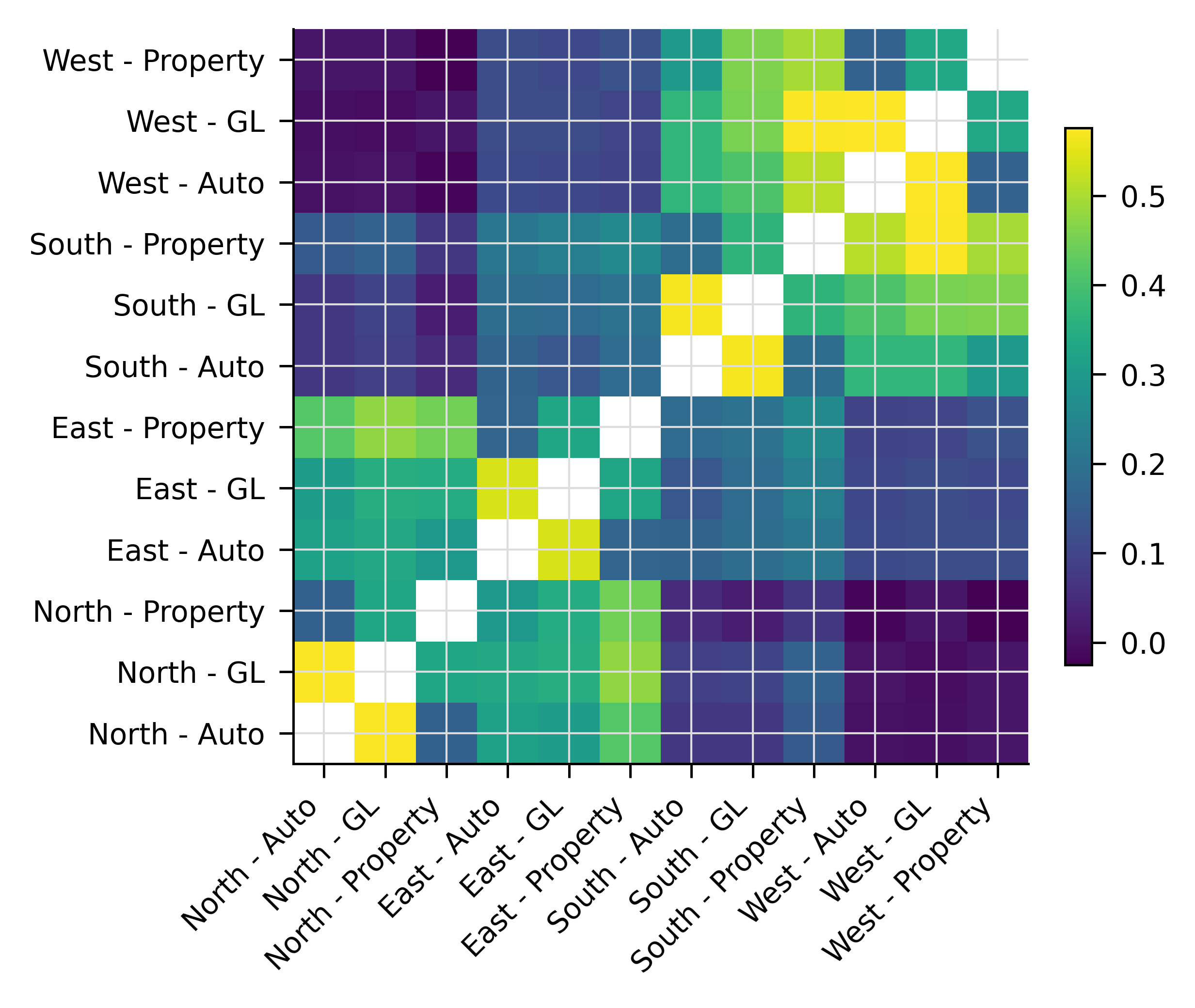
Table 8.7 shows the overall correlation matrix at the line-region level (12 x 12 matrix), and Figure 8.4 shows an image plot of the same matrix. The underlying block structure is clear from the image.
| index | N-AL | N-GL | N-Pr | E-AL | E-GL | E-Pr | S-AL | S-GL | S-Pr | W-AL | W-GL | W-Pr |
|---|---|---|---|---|---|---|---|---|---|---|---|---|
| N-AL | 1 | 0.573 | 0.162 | 0.320 | 0.304 | 0.419 | 0.072 | 0.073 | 0.145 | 0.003 | -0.000 | 0.012 |
| N-GL | 0.573 | 1 | 0.332 | 0.338 | 0.349 | 0.476 | 0.089 | 0.099 | 0.163 | 0.007 | -0.005 | 0.011 |
| N-Pr | 0.162 | 0.332 | 1 | 0.296 | 0.346 | 0.448 | 0.052 | 0.022 | 0.073 | -0.017 | 0.011 | -0.025 |
| E-AL | 0.320 | 0.338 | 0.296 | 1 | 0.539 | 0.170 | 0.167 | 0.190 | 0.211 | 0.109 | 0.118 | 0.118 |
| E-GL | 0.304 | 0.349 | 0.346 | 0.539 | 1 | 0.329 | 0.137 | 0.186 | 0.233 | 0.105 | 0.116 | 0.107 |
| E-Pr | 0.419 | 0.476 | 0.448 | 0.170 | 0.329 | 1 | 0.184 | 0.201 | 0.257 | 0.098 | 0.100 | 0.128 |
| S-AL | 0.072 | 0.089 | 0.052 | 0.167 | 0.137 | 0.184 | 1 | 0.567 | 0.188 | 0.371 | 0.370 | 0.301 |
| S-GL | 0.073 | 0.099 | 0.022 | 0.190 | 0.186 | 0.201 | 0.567 | 1 | 0.365 | 0.409 | 0.456 | 0.460 |
| S-Pr | 0.145 | 0.163 | 0.073 | 0.211 | 0.233 | 0.257 | 0.188 | 0.365 | 1 | 0.512 | 0.573 | 0.495 |
| W-AL | 0.003 | 0.007 | -0.017 | 0.109 | 0.105 | 0.098 | 0.371 | 0.409 | 0.512 | 1 | 0.576 | 0.164 |
| W-GL | -0.000 | -0.005 | 0.011 | 0.118 | 0.116 | 0.100 | 0.370 | 0.456 | 0.573 | 0.576 | 1 | 0.332 |
| W-Pr | 0.012 | 0.011 | -0.025 | 0.118 | 0.107 | 0.128 | 0.301 | 0.460 | 0.495 | 0.164 | 0.332 | 1 |
8.2.8 Theoretical derivation of the Iman-Conover method
Suppose that \(\mathsf{M}\) is an \(n\) element sample from an \(r\) dimensional multivariate distribution, so \(\mathsf{M}\) is an \(n\times r\) matrix. Assume that the columns of \(\mathsf{M}\) are uncorrelated, have mean zero, and have a standard deviation of one. Let \(\mathsf{M}'\) denote the transpose of \(\mathsf{M}\). These assumptions imply that the correlation matrix of the sample \(\mathsf{M}\) can be computed as \(n^{-1}\mathsf{M}'\mathsf{M}\), and because the columns are independent, \(n^{-1}\mathsf{M}'\mathsf{M}=\mathsf{id}\). (There is no need to scale the covariance matrix by the row and column standard deviations because they are all one. In general \(n^{-1}\mathsf{M}'\mathsf{M}\) is the covariance matrix of \(\mathsf{M}\).)
Let \(\mathsf{S}\) be a correlation matrix, i.e., \(\mathsf{S}\) is a positive semidefinite symmetric matrix with ones on the diagonal and all elements \(\le 1\) in absolute value. In order to rule out linearly dependent variables, assume \(\mathsf{S}\) is positive definite. These assumptions ensure \(\mathsf{S}\) has a Choleski decomposition \[ \mathsf{S}=\mathsf{C}'\mathsf{C} \] for some upper triangular matrix \(\mathsf{C}\), see Golub and Van Loan (2013) or Press et al. (1992). Set \(\mathsf{T}=\mathsf{M}\mathsf{C}\). The columns of \(\mathsf{T}\) still have mean zero, because they are linear combinations of the columns of \(\mathsf{M}\), which have zero mean by assumption. It is less obvious, but still true, that the columns of \(\mathsf{T}\) still have standard deviation one. To see why, remember that the covariance matrix of \(\mathsf{T}\) is \[ n^{-1}\mathsf{T}'\mathsf{T}=n^{-1}\mathsf{C}'\mathsf{M}'\mathsf{M}\mathsf{C}=\mathsf{C}'\mathsf{C}=\mathsf{S}, \tag{8.2}\] since \(n^{-1}\mathsf{M}'\mathsf{M}=\mathsf{id}\) is the identity by assumption. Now \(\mathsf{S}\) also is actually the correlation matrix because the diagonal is scaled to standard deviation one, so the covariance and correlation matrices coincide. The process of converting \(\mathsf{M}\), which is easy to simulate, into \(\mathsf{T}\), which has the desired correlation structure \(\mathsf{S}\), is the theoretical basis of the Iman-Conover method.
It is important to note that estimates of correlation matrices, depending on how they are constructed, need not have the mathematical properties of a correlation matrix. Therefore, when trying to use an estimate of a correlation matrix in an algorithm, such as the Iman-Conover, which actually requires a proper correlation matrix as input, it may be necessary to check the input matrix does have the correct mathematical properties.
Next, we discuss how to make \(n\times r\) matrices \(\mathsf{M}\), with independent, mean zero columns. The basic idea is to take \(n\) numbers \(a_1,\dots,a_n\) with \(\sum_i a_i=0\) and \(n^{-1}\sum_i a_i^2=1\), use them to form one \(n\times 1\) column of \(\mathsf{M}\), and then to copy it \(r\) times. Finally, randomly permute the entries in each column to make them independent as columns of random variables. Iman and Conover call these \(a_i\) scores. They discuss several possible definitions for scores, including scaled versions of \(a_i=i\) (ranks) and \(a_i\) uniformly distributed. They note that the shape of the output multivariate distribution depends on the scores. All of the examples in their paper use normal scores.
Given that the scores will be based on normal random variables, we can either simulate \(n\) random standard normal variables and then shift and rescale to ensure mean zero and standard deviation one, or we can use a systematic sample from the standard normal, \(a_i=\Phi^{-1}(i/(n+1))\). By construction, the systematic sample has mean zero, which is an advantage. Also, by symmetry, using the systematic sample halves the number of calls to \(\Phi^{-1}\). For these two reasons we prefer it in the algorithm below.
The correlation matrix of \(\mathsf{M}\), constructed by randomly permuting the scores in each column, will only be approximately equal to \(\mathsf{id}\) because of random simulation error. In order to correct for the slight error which could be introduced, Iman and Conover use another adjustment in their algorithm. Let \(\mathsf{EE}=n^{-1}\mathsf{M}'\mathsf{M}\) be the actual correlation matrix of \(\mathsf{M}\), and let \(\mathsf{EE}=\mathsf{F}'\mathsf{F}\) be the Choleski decomposition of \(\mathsf{EE}\), and define \(\mathsf{T}=\mathsf{M}\mathsf{F}^{-1}\mathsf{C}\). The columns of \(\mathsf{T}\) have mean zero, and the covariance matrix of \(\mathsf{T}\) is \[ \begin{aligned} n^{-1}\mathsf{T}'\mathsf{T} &= n^{-1}\mathsf{C}'\mathsf{F}'^{-1}\mathsf{M}'\mathsf{M}\mathsf{F}^{-1}\mathsf{C} \notag \\ &= \mathsf{C}'\mathsf{F}'^{-1}\mathsf{EE}\mathsf{F}^{-1}\mathsf{C} \notag \\ &= \mathsf{C}'\mathsf{F}'^{-1}\mathsf{F}'\mathsf{F}\mathsf{F}^{-1}\mathsf{C} \notag \\ &= \mathsf{C}' \mathsf{C} \notag \\ &= \mathsf{S} \end{aligned} \] and hence \(\mathsf{T}\) has correlation matrix exactly equal to \(\mathsf{S}\), as desired. If \(\mathsf{EE}\) is singular, then the column shuffle needs to be repeated.
Now that the reference distribution \(\mathsf{T}\) with exact correlation structure \(\mathsf{S}\) is in hand, all that remains to complete the Iman-Conover method is to reorder each column of the input distribution \(\mathsf{X}\) to have the same rank order as the corresponding column of \(\mathsf{T}\).
8.3 Allocating capital, if you must
Within each layer, we can allocate its expected losses and premiums to the various portfolio units. Having done so, capital allocation to units follows.
Admonition. We can’t emphasize strongly enough that you should not allocate capital. Different layers of capital do not have the same cost (think: equity, junk debt, government bonds), therefore you do not know the appropriate target return on your allocated capital. Without that, you can’t say if a projected return is good or bad. Allocate margin, not capital!
Warnings about smoking don’t work either. We know your CFO, senior management, and investors discuss allocating underwriting capacity in the language of allocating capital, and we previously admonished you to speak the language of your customers. This section describes two methods you can use to translate allocated margins into allocated capital.
The first method is obvious: simply assume all capital earns the weighted average cost of capital and allocate capital by dividing allocated margin by the weighted average cost of capital. This will result in an additive allocation of capital. This has the advantage of being simple to implement, but the disadvantage is that it obscures—nay, denies!—the fact that different segments of capital earn different returns.
The second method has a more theoretically sound basis. It applies the principles discussed in Chapter 4 to obtain an allocation of capital \(Q\) and unit-specific rates of return \(\iota^i\) consistent with the SRM approach.
Layer \(k\) is \(\Delta X_k\) dollars wide but is triggered by any portfolio loss \(X > X_k\). We propose that the expectation of that loss be allocated to units by equal priority, that is, in proportion to the expected losses of the units in those triggering events. We may define the layer-\(k\) expected loss share to unit \(i\) as \[ \alpha_k^i := \mathsf E_p\left[\frac{X^i}{X}\mid X > X_k\right]. \] In particular, this means \[ \alpha_k^i S_k = \mathsf E_p\left[\frac{X^i}{X}1_{\mid X > X_k}\right] = \sum_{j>k}\frac{X_j^i}{X_j}p_j. \tag{8.3}\] The \(\alpha^i\) sum to one across the units because (conditional) expectations are linear. The expected loss to layer \(k\), \(S_k\Delta X_k\), can thus be partitioned into \(\alpha_k^i S_k\Delta X_k\) across the various units. The total portfolio loss, \(\mathsf E[X]\), is allocated to unit \(i\) as \[ \mathsf E[X^i] = \sum_j \alpha_j^i S_j\Delta X_j. \tag{8.4}\]
Exercise. Prove Equation 8.4, given Equation 8.3.
Solution. \[ \begin{aligned} \sum_j \alpha_j^i S_j\Delta X_j &= \sum_{k=0}^{n-1} \left(\sum_{j=k+1}^{n}\frac{X_j^i}{X_j} p_j \right)(X_{k+1}-X_k) \\ &=\sum_{j=1}^n \frac{X_j^i}{X_j} p_j\sum_{k=0}^{j-1} (X_{k+1}-X_{k}) \\ &=\sum_{j=1}^n \frac{X_j^i}{X_j} p_j X_j \\ &=\sum_{j=1}^n X_j^i p_j \\ &= \mathsf E[X^i] \end{aligned} \] noting \(X_0=X_0^i=0\).
What about premium? We propose that the premium associated with layer \(k\) be allocated to units in proportion to the distorted expected losses of the units in those triggering events. This leads to the definition of the distorted expected loss share \[ \beta_k^i := \mathsf E_q\left[\frac{X^i}{X}\mid X > X_k\right] \] In particular, this means \[ \beta_k^i g(S_k) = \sum_{j>k}\frac{X_j^i}{X_j}q_j = \sum_{j>k}\frac{X_j^i Z_j}{X_j}p_j. \] where, recall, \(Z_j=q_j/p_j\) is the event weight.
The premium to layer \(k\), given by \(P_k = g(S_k)\Delta X_k\), is partitioned to the units as \(\beta_k^i g(S_k)\Delta X_k\). The total premium is therefore allocated to the units as \[ \mathsf E[X^i Z(X)] = \sum_j \beta_j^i g(S_j)\Delta X_j \] being the total premium to unit \(i\).
Exercise. Prove the previous equality.
Solution. The same steps as the preceding exercise.
Since margin is the difference between premium and expected loss (Equation 4.1), we immediately have the allocation of unit \(i\)’s margin \[ M^i = \sum_j (\beta_j^i g(S_j) - \alpha_j^i S_j)\Delta X_j. \tag{8.5}\]
Exercise. Use Equation 4.10 with Equation 4.8 and Equation 4.9 to derive a simple equation for \(M^i\) and then prove it is the equivalent of Equation 8.5.
Recall that the layer \(k\) cost of capital is \[ \iota_k := \frac{M_k}{Q_k} = \frac{P_k - S_k\Delta X_k}{\Delta X_k-P_k} = \frac{g(S_k) - S_k}{1- g(S_k)}. \] Here, we lean on the assumption of law invariance (see Section 4.4). We claim that for a law invariant pricing approach, the layer cost of capital must be the same for all units. Law invariance implies the risk measure is only concerned with the attachment probability of the layer and not with the cause of loss within the layer. If \(\iota\) within a layer varied by unit, then the allocation could not be law invariant. This crucial observation underlies the following logic.
Because cost of capital equals margin over capital, and seeing as both margin and cost of capital are known by layer and by unit, with the latter constant across units, we can compute unit capital by layer \(Q_k^i\) via
\[\begin{equation} \iota_k: = \frac{M_k}{Q_k} = \frac{M_k^i}{Q_k^i}\implies Q_k^i = \frac{M_k^i}{\iota_k}. \end{equation}\] Substituting the details gives the following definition for the NA of capital in layer \(k\) to unit \(i\): \[ Q_k^i = \frac{\beta_k^i g(S_k) - \alpha_k^i S_k}{g(S_k)- S_k} (1-g(S_k))\Delta X_k. \tag{8.6}\]
In words, taking Equation 8.6 and dividing numerator and denominator by capital in the layer shows \[ Q_k^i = \frac{\text{Margin for unit in layer}}{\text{Total margin in layer}}\times \text{Capital in layer} = \frac{\text{Margin for unit in layer}}{\text{Layer cost of capital}}. \] The NA is the same as method 1 (divide by weighted average cost of capital) but applied separately for each layer of capital!
Exercise. Derive Equation 8.6.
Since \(1-g(S_k)\) is the proportion of of layer \(k\)’s limit devoted to capital, this says the proportion of capital allocated to unit \(i\) is given by the nicely symmetric expression \[ \frac{\beta_k^i g(S_k) - \alpha_k^i S_k}{g(S_k)- S_k} \tag{8.7}\] To determine total capital by unit, we sum across layers \[ Q^i := \sum_j Q_j^i. \] Finally, we can determine the average cost of capital for unit \(i\) \[\begin{equation} \iota^i = \frac{M^i}{Q^i}. \end{equation}\]
This is illustrated for our example in Table 8.8, Table 8.9, and Table 8.10. In the last table, the columns are calculated as \(M^i=\beta^i g(S)-\alpha^i S\), \(\iota=(g-S)/(1-g)\), \(Q^i=M^i/\iota\), and the low row \(M\) (respectively, \(Q\)) show sum products with \(\Delta X\).
| \(k\) | Unit A \(X^1\) | Unit B \(X^2\) | Unit C \(X^3\) | Total \(X\) | \(p\) | \(S\) | \(\Delta X\) | \(\alpha^1 S\) | \(\alpha^2 S\) | \(\alpha^3 S\) |
|---|---|---|---|---|---|---|---|---|---|---|
| 0 | 0 | 0 | 0 | 0 | 0 | 1 | 22 | 0.325 | 0.441 | 0.234 |
| 1 | 15 | 7 | 0 | 22 | 0.1 | 0.9 | 6 | 0.257 | 0.409 | 0.234 |
| 2 | 15 | 13 | 0 | 28 | 0.1 | 0.8 | 8 | 0.203 | 0.362 | 0.234 |
| 3 | 5 | 20 | 11 | 36 | 0.1 | 0.7 | 4 | 0.189 | 0.307 | 0.204 |
| 4 | 10 | 24 | 6 | 40 | 0.4 | 0.3 | 15 | 0.089 | 0.067 | 0.144 |
| 5 | 26 | 19 | 10 | 55 | 0.1 | 0.2 | 10 | 0.042 | 0.032 | 0.126 |
| 6 | 17 | 8 | 40 | 65 | 0.1 | 0.1 | 35 | 0.016 | 0.020 | 0.064 |
| 7 | 16 | 20 | 64 | 100 | 0.1 | 0 | 0 | 0 | 0 | 0 |
| \(L=\mathsf E_p\) | 13.4 | 18.3 | 14.9 | 46.6 | 13.4 | 18.3 | 14.9 |
| \(k\) | Unit A \(X^1\) | Unit B \(X^2\) | Unit C \(X^3\) | Total \(X\) | \(q\) | \(gS\) | \(\Delta X\) | \(\beta^1 S\) | \(\beta^2 S\) | \(\beta^3 S\) |
|---|---|---|---|---|---|---|---|---|---|---|
| 0 | 0 | 0 | 0 | 0 | 0 | 1 | 22 | 0.295 | 0.409 | 0.296 |
| 1 | 15 | 7 | 0 | 22 | 0.052 | 0.948 | 6 | 0.260 | 0.392 | 0.296 |
| 2 | 15 | 13 | 0 | 28 | 0.066 | 0.882 | 8 | 0.225 | 0.362 | 0.296 |
| 3 | 5 | 20 | 11 | 36 | 0.075 | 0.807 | 4 | 0.214 | 0.320 | 0.273 |
| 4 | 10 | 24 | 6 | 40 | 0.379 | 0.428 | 15 | 0.119 | 0.093 | 0.216 |
| 5 | 26 | 19 | 10 | 55 | 0.119 | 0.309 | 10 | 0.063 | 0.051 | 0.194 |
| 6 | 17 | 8 | 40 | 65 | 0.135 | 0.174 | 35 | 0.028 | 0.035 | 0.111 |
| 7 | 16 | 20 | 64 | 100 | 0.174 | 0 | 0 | 0 | 0 | 0 |
| \(L=\mathsf E_p\) | 13.4 | 18.3 | 14.9 | 46.6 | ||||||
| \(P=\mathsf E_p\) | 14.109 | 18.637 | 20.819 | 53.565 | 14.109 | 18.637 | 20.819 | |||
| \(M=P-L\) | 0.709 | 0.337 | 5.919 | 6.965 |
| \(k\) | Total \(X\) | \(\Delta X\) | \(M^1\) | \(M^2\) | \(M^3\) | \(Q^1\) | \(Q^2\) | \(Q^3\) | \(\iota\) | \(\delta\) |
|---|---|---|---|---|---|---|---|---|---|---|
| 0 | 0 | 22 | -0.030 | -0.032 | 0.061 | 0 | 0 | 0 | inf | 1 |
| 1 | 22 | 6 | 0.003 | -0.017 | 0.061 | 0.003 | -0.018 | 0.067 | 0.917 | 0.478 |
| 2 | 28 | 8 | 0.021 | -0.001 | 0.061 | 0.031 | -0.001 | 0.089 | 0.693 | 0.409 |
| 3 | 36 | 4 | 0.025 | 0.013 | 0.069 | 0.045 | 0.024 | 0.125 | 0.555 | 0.357 |
| 4 | 40 | 15 | 0.030 | 0.026 | 0.072 | 0.134 | 0.115 | 0.323 | 0.224 | 0.183 |
| 5 | 55 | 10 | 0.021 | 0.019 | 0.069 | 0.133 | 0.121 | 0.437 | 0.158 | 0.136 |
| 6 | 65 | 35 | 0.012 | 0.015 | 0.047 | 0.132 | 0.165 | 0.529 | 0.089 | 0.082 |
| 7 | 100 | 0 | 0 | 0 | 0 | 0 | 0 | 0 | ||
| \(\mathsf E_q\) | 0.709 | 0.337 | 5.919 | 8.411 | 8.691 | 29.333 | ||||
| \(\iota\) | 0.084 | 0.039 | 0.202 | 0.150 |
Observe that \((\sum_i \iota^i Q^i)/Q\) is 15%, the weighted cost of capital over all units is 15%, as assumed.
Notice that the first layer \(k=0\) has undefined cost of capital \(\iota\); since \(S_0=1\), we have \(g(S_0)=1\), \(P_0=\Delta X_0\), and \(M_0=Q_0=0\). Nonetheless, we have nonzero unit margins \(M_0^i\) summing to zero.
The smallest portfolio loss equals 22, meaning the first layer is entirely funded by loss payments and requires no capital in aggregate. However, there are cross-subsidies between the units within the layer. Were the three units to purchase insurance from an insurance company with only $22 of assets, it would benefit the most volatile line, because it would capture an outsized proportion of the available assets in the case it had a large loss. The margins reflect these cross-subsidies. However because the layer is fully funded by losses, there is no capital and hence no aggregate margin, which is why the allocated margins sum to zero.
Although the cost of capital within each layer is the same for all units, the margin, the proportion of limit that is capital, and the proportion of that capital attributable to each unit, all vary across layers. Therefore, average cost of capital generally varies by unit. Table 8.11 shows the difference in results between the natural Wang allocation and the CCoC approaches done previously. (The natural CCoC is equivalent to the industry standard approach.) The story is complex. While both noncatastrophe lines receive more margin and more capital under the Wang allocation, it is not proportional; their rates of return are not only lower than the 15% benchmark, but they are markedly different.
| Distortion | Metric | Unit A | Unit B | Unit C | Portfolio |
|---|---|---|---|---|---|
| Wang, 0.343 | Capital \(Q\) | 8.411 | 8.691 | 29.333 | 46.435 |
| Margin \(M\) | 0.709 | 0.337 | 5.919 | 6.965 | |
| Return \(\iota\) | 8.4% | 3.9% | 20.2% | 15.0% | |
| CCoC, 0.150 | Capital \(Q\) | 4.874 | 5.288 | 36.273 | 46.435 |
| Margin \(M\) | 0.339 | 0.222 | 6.404 | 6.965 | |
| Return \(\iota\) | 7.0% | 4.2% | 17.7% | 15.0% |
For a typical distortion other than CCoC, in line with Table 1.1, we find:
- Lower layers of assets, below the expected losses, have a high cost of capital but, offsetting this, they are mostly funded by premium and require little supporting investor capital, resulting in high leverage.
- Higher layers of assets have a lower cost of capital but higher capital content: they are funded by capital to a greater degree.
- Low volatility units by definition tend to have losses close to their expected value, regardless of the value of total losses, and so consume relatively more of the expensive, lower layer capital and a smaller proportion of cheaper, higher asset layers. Offsetting this, there is more capital in higher layers than lower ones.
- High volatility units tend to have a larger proportion of total losses when the portfolio total loss is large, and so they consume a greater proportion of cheaper, higher layer capital.
We see all of these phenomena in the example.
With price, quantity, and proportion all variable the overall effect of the NA of capital is hard to predict. Since price, amount, and use are all correlated, it is never adequate to assume that the unit average cost of capital is the portfolio average cost of capital. This is the fundamental flaw in the industry standard approach, which uses the same cost of capital for all capital layers (see Section 4.7). The SRM-based method outlined here produces varying cost of capital by unit in a defensible manner—given a choice of distortion function. How to make that choice was discussed in Chapter 6.
8.4 Comparions with Bodoff’s layer capital allocation
Readers may have guessed that the NA is closely related to Bodoff’s layer capital allocation (Bodoff 2007). This section will explain how they are correct and show the connections, similarities, and differences between the two approaches. Bodoff’s approach uses \(\alpha^i\), which describes how loss in each layer is shared between the units, and applies it to all assets in the layer. Since \(\sum_i \alpha^1 = 1\) we get a decomposition \[ a = \int_0^a 1\,dx = \sum_i \int_0^a \alpha^i(x)\,dx. \] Thus, \(a^i=\int_0^a \alpha^i(x)\,dx\) is a reasonable allocation of assets. However, to determine a premium \(a^i\) needs to be split into amounts \(P^i + Q^i\) funded by policyholder premium and investor capital. For example, we could fall back to CCoC, resulting in a layer premium \[ (\alpha^i(x) S(x) + \delta \alpha^i(x) (1 - S(x))) + \nu \delta \alpha^i(x) (1 - S(x)) \] where the first parenthetic term is expected loss (Equation 8.3) plus a margin \(\delta\) times the unfunded liability (Table 4.1, P3), and the second term is investor capital (Table 4.1, Q). This reproduces distortion CCoC pricing. Picking other distortions, which allow for the unfunded liability to be split differently than losses, produces a range of other answers. Bodoff’s paper is very insightful, but it falls short by not fully describing a premium allocation: further assumptions are still needed to convert allocated assets into allocated premiums. Table 8.12 shows Bodoff’s asset allocation in the last four right-hand columns.
| \(k\) | Total \(X\) | \(p\) | \(S\) | \(\Delta X\) | \(\alpha^1\Delta X\) | \(\alpha^2\Delta X\) | \(\alpha^3\Delta X\) | \(\sum\alpha^i\Delta X\) |
|---|---|---|---|---|---|---|---|---|
| 0 | 0 | 0 | 1 | 22 | 7.152 | 9.694 | 5.154 | 22 |
| 1 | 22 | 0.1 | 0.9 | 6 | 1.713 | 2.726 | 1.562 | 6 |
| 2 | 28 | 0.1 | 0.8 | 8 | 2.033 | 3.624 | 2.343 | 8 |
| 3 | 36 | 0.1 | 0.7 | 4 | 1.082 | 1.753 | 1.164 | 4 |
| 4 | 40 | 0.4 | 0.3 | 15 | 4.471 | 3.343 | 7.186 | 15.000 |
| 5 | 55 | 0.1 | 0.2 | 10 | 2.108 | 1.615 | 6.277 | 10.000 |
| 6 | 65 | 0.1 | 0.1 | 35 | 5.600 | 7.000 | 22.400 | 35.000 |
| 7 | 100 | 0.1 | 0 | 0 | 0 | 0 | 0 | 0 |
| Total | 46.6 | 24.159 | 29.756 | 46.086 | 100.0 |